
. Introduction
Manas Lake is a closed lake basin located in the western part of the Junggar Basin in northern Xinjiang Province, northwestern China. It is adjacent to Gurbantunggut Desert to the east (Fig. 1). The lake is elongated in the NE-SW direction (Fig. 2), and its current lake bed is at an elevation of 244 m a.s.l. As hydrological systems in such arid region are sensitive to climate change, valuable information about the paleoenvironmental changes can be obtained through studies of sedimentary records in Manas Lake. Understanding past changes of the lake is important in predicting future hydrological changes, as well as managing water resources in the region.
Fig. 1
Map of northern Xinjiang showing the major water systems, including the Manas Lake west of the Gurbantunggut Desert. Inset map shows the northern Xinjiang area (in dotted rectangle) and the present wind systems in Asia (Herzschuh, 2006).
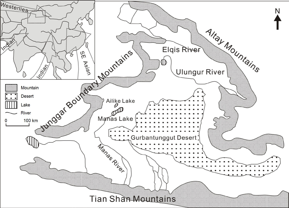
Fig. 2
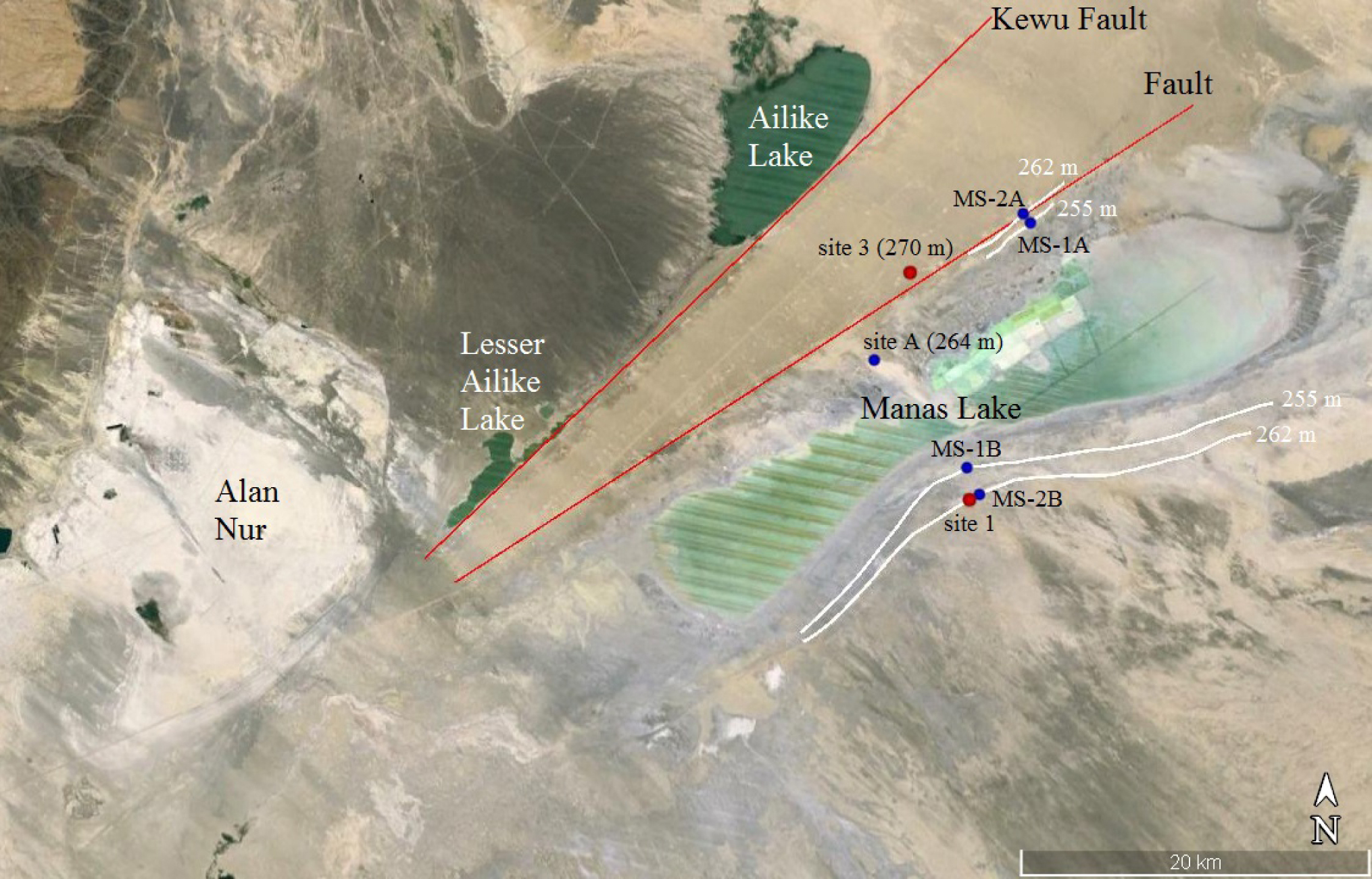
Google Earth image showing the Manas Lake area and two NE-trending faults. Sampling locations for this study (red dots) and for previous studies by Fan et al. (2012) and Wang (2014) (blue dots) are also shown, together with paleoshorelines (white lines). The elevation shown is in meters above sea level.
In previous studies on Manas Lake, radiocarbon dating (e.g. Rhodes et al., 1996) and optically stimulated luminescence (OSL) dating (e.g. Li and Fan, 2011; Fan et al., 2012; Wang, 2014) have been used to obtain a detailed chronology for paleoenvironmental changes. Based on radiocarbon dating, Rhodes et al. (1996) studied sedimentary cores near the center of Manas Lake, and suggested that there was a humid period during 42–36 ka cal BP, followed by an extreme dry phase during the Last Glacial Maximum. It was also suggested that the climate in the region has become wetter again since ~10 ka ago, but was interrupted with dry phases (Rhodes et al., 1996). However, radiocarbon dating requires carbon-rich materials which are not common in Manas Lake sediments, and may suffer from old carbon contamination (e.g. Wang et al., 2002). In contrast, OSL dating can be applied directly to quartz or K-feldspar grains in sediments, and has a slight advantage of higher datable age limits.
Using OSL dating, Fan et al. (2012) dated a sedimentary section at site A (Fig. 2) on northwestern side of the lake at an elevation of 264 m a.s.l. (~20 m above lake bed). Based on the OSL ages of lacustrine sediments with variations in depositional facies, they interpreted that high lake levels (higher than site A) existed before ~66 ka ago and during ~38–27 ka ago. These two periods correspond to the relatively warm and humid period during marine isotope stage 5 (MIS 5) and late MIS 3 respectively. Additionally, there was a stage of relatively stable lake level at or slightly below site A during ~48–44 ka ago, corresponding to MIS 3b. At this period, site A was at or near a paleoshoreline environment. There were no sedimentary records during ~64–48 ka ago and between ~27 ka ago and the recent time at site A (Fan et al., 2012).
Later, Wang (2014) focused on dating young, late Holocene sediments of Manas Lake. He identified two paleoshoreline terraces at elevation 255 and 262 m a.s.l. (11 and 18 m above lake bed respectively) on both northwestern and southeastern sides of the lake (Fig. 2). He obtained an OSL age of ~300 a for the upper paleoshoreline (sites MS-2A and MS-2B), while the lower paleoshoreline (sites MS-1A and MS-1B) was too young to be OSL-dated. This suggests a cold and wet Little Ice Age, when the lake level once reached ~262 m a.s.l., forming the upper paleoshoreline. The lake level then dropped steadily towards the present, with the lower paleoshoreline (255 m) formed more recently (within the last century) due to a short period of stable lake level (Wang, 2014). Manas Lake became completely dried in 1962, only being recovered occasionally in summer after 1999 (Zhang and Li, 2004).
Wang (2014) also found a sedimentary break in his sampling section of the upper paleoshoreline in the southeastern side (MS-2B of Fig. 2) of Manas Lake, in which the sample from the layer beneath the Little Ice Age sediments gives a much stronger natural OSL signal. Similar to the results of Fan et al. (2012), there are no shoreline or lacustrine sediment records of a high lake level between the Little Ice Age and MIS 3 in his studied sites. The sedimentary break indicates that large-scale erosion may have occurred in the area. It is not known the size of the age gap represented in Wang’s (2014) southeastern paleoshoreline section. Also, previous studies on older sediments in the area only focused on northwestern side of the lake (Fan et al., 2012). It is therefore necessary to take samples again from the southeastern side for OSL dating, in order to allow comparison between the two sides of the lake at similar elevation. Besides that, a well-exposed sedimentary section on the northwestern side of the lake will also be studied and dated to further understand the paleoenvironmental changes. Comparison with previous results will be made, and the implications on the climatic and tectonic evolution of the lake will be discussed.
. Geological and geomorphological setting
Adjacent to the Gurbantunggut Desert (Fig. 1), the regional climate is arid, and is dominantly controlled by the Westerlies (Wang et al., 2005). The area has a mean annual precipitation of 64 mm and a mean annual evaporation of 3110 mm (Yao et al., 2007). Despite such an arid condition, Manas Lake once had a lake surface area of 550 km2 (60–70 km long and 10–20 km wide) and an average water depth of 6 m in 1957 (Zhang and Li, 2004). At that time, it was supported by Manas River in the south (Fig. 1). Due to intensified agricultural activities which used water intensively, the Manas River was cut off at its lower course and it could not reach Manas Lake (Cheng et al., 2001; Zhang and Li, 2004). As a result, the lake became completely dried in 1962 (Zhang and Li, 2004). As the saline lake dried up, evaporite deposits were formed on the lake bed, which have been exploited for halite. After 1999, Mana River can occasionally reach Manas Lake again. At present, Manas Lake is an intermittent lake occasionally supported by Manas River, as well as groundwater discharge (Zhang and Li, 2004; Yao and Li, 2010).
Previous geomorphological studies show that Manas Lake is a remnant of a much larger lake, called the Paleo-Manas Lake. The large lake was a wandering lake, originally formed due to tectonic subsidence in the western part of Junggar Basin in the early Pleistocene (Wang, 1991). Based on the distribution of lacustrine sediments and satellite data, the lake level once reached ~93 m above the present Manas Lake bed (Fan et al., 2012). It was supported by various rivers in the region, including Ulungur River and Elqis River from the north, and other river systems originating from glaciers in Tian Shan in the south, such as the Manas River (Fig. 1). But in the later part of the Pleistocene, Ulungur River and Elqis River stopped flowing to the lake due to tectonic movements. As a result, the lake level dropped and the Paleo-Manas Lake broke up into several lakes (Zhou, 1963; Mu et al., 2001; Yang and Shi, 2003; Yao and Li, 2010). These include the modern Manas Lake, Ailike Lake, Lesser Ailike Lake and the dried Alan Nur (Fig. 2).
It is noted that the evolution of Manas Lake was controlled not only by climate change, but also neotectonic activities (Wang, 1991; Mu et al., 2001; Shi et al., 2008; Yao and Li, 2010). It has been suggested that faulting activities have caused differential uplift in the region quite recently (Yao and Li, 2010, Gong et al., 2015; Fu et al., 2017). Some of these faults can be identified on Google Earth Image (Fig. 2). Reports suggested that the course change of Manas River in 1915 and the subsequent drying up of Alan Nur were related to the uplift, although blocking of river channel by sedimentation is believed to be the main reason of such changes (Zhang and Li, 2004; Shi et al., 2008; Gong et al., 2014). Uplifting may lead to false interpretation of the past lake level and thus the paleoenvironment. It is therefore important to understand the spatial extent and the timing of neotectonic activities in the area, before a detailed paleoenvironmental change can be inferred.
. Sampling and laboratory procedures
Sampling sites
Samples were collected from two sites in Manas Lake (sites 1 and 3 on Fig. 2). OSL samples were taken either by hammering stainless steel tubes (30-cm long with 5-cm diameter) into an exposed sedimentary section (site 1), or by taking block samples (site 3). Both ends of the tubes were then sealed immediately with tissue papers and tapes to avoid any exposure to light or loss of moisture content. For block samples, they were sealed in plastic bags and were wrapped with tapes to avoid breakage during transport.
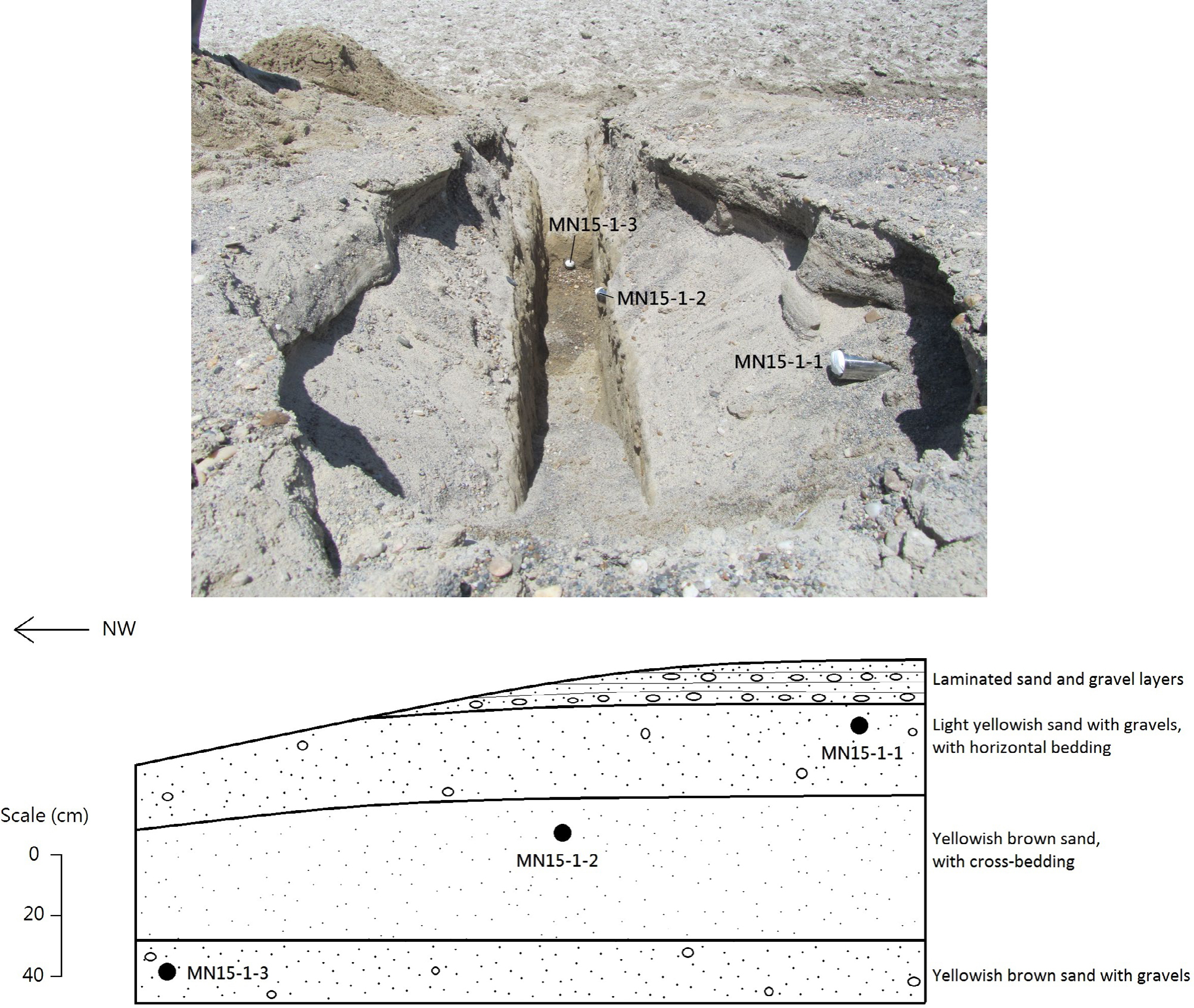
Site 1 (45°44′53.1″N, 85°55′16.6″E) is located on the upper paleoshoreline in the southeastern side of Manas Lake at an elevation of 262 m a.s.l. This site is close to Wang’s (2014) section (MS-2B) along the paleoshoreline terrace. A trench was dug to expose a sedimentary section of ~1 m deep (Fig. 3). The 15 cm-thick top layer of the section consists of dark greyish rounded granules and pebbles interbedded with light yellowish coarse sand containing occasional granules. They were likely deposited in recent flooding events. The next ~30 cm is made of horizontally-bedded light yellowish coarse sand with small amount of sub-rounded gravels. It is the same layer as Wang’s (2014) paleoshoreline sample, and is expected to have an age of a few centuries based on the OSL date by Wang (2014). This is underlain by ~40 cm thick of cross-bedded yellowish brown medium to coarse sand, which is finer and wetter than the light yellowish sand above. The relatively coarse grain size of sand indicates a near-shore environment, with a paleo-current dominantly flowing to the center of the lake as indicated by cross-bedding. This layer is further underlain by relatively wet, yellowish brown coarse sand with some sub-rounded gravels at the bottom of the section. The coarse-grain nature again indicates an environment near a paleoshoreline. OSL samples were collected from each of the three sandy layers (Fig. 3). The purpose of dating these samples is to establish the size of the sedimentary age gap described in section 1, in the southeastern side of Manas Lake. It also helps to determine the time when relatively wet episodes occurred in the lake area.
Fig. 3
Field photo showing the excavated trench at paleoshoreline site 1, and the schematic diagram of the section.
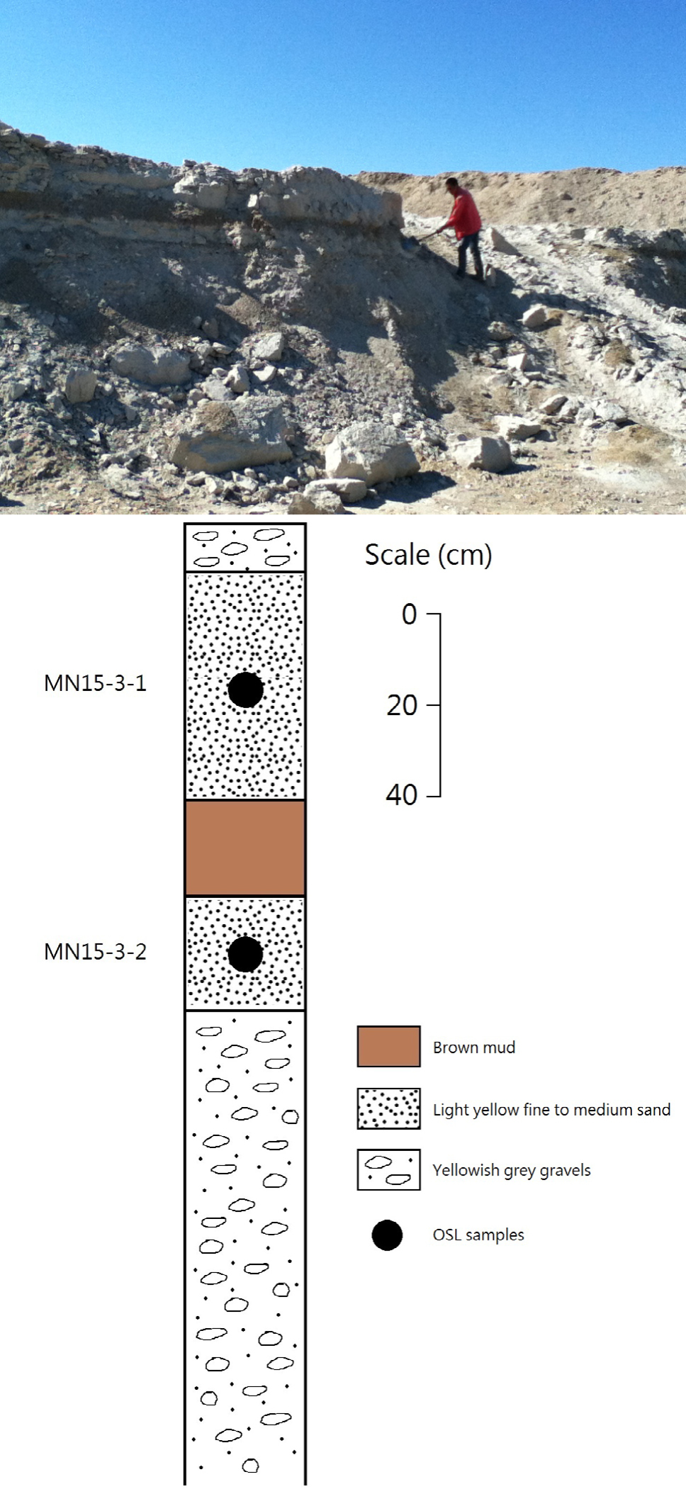
Site 3 (45°51′51.6″N, 85°52′38.6″E) is located on the northwestern side of Manas Lake at an elevation of 270 m a.s.l. An exposed vertical sedimentary section was found (Fig. 4). The top of the section is a thin layer of yellowish grey gravels, indicating a fluvial environment. The next ~55 cm of the section consists of very light yellowish fine to medium sand. The relatively fine-grain nature of the sand suggests an offshore shallow lacustrine environment. It is underlain by a ~20 cm thick layer of brown mud. The brownish color indicates an oxidizing environment. Thus, the brown mud was likely deposited in a very shallow and quiet water environment, occasionally exposed to the air. Below the muddy layer, there is another ~25 cm thick layer of very light yellowish fine to medium sand, which indicates a shallow lacustrine environment again. The bottom of the section is made of yellowish grey, poorly sorted fluvial gravels (dominantly pebbles and granules), which is more than 2 m thick. OSL samples were collected from the middle of each of the two sandy layers (Fig. 4). As it was too hard for hammering stainless steel tube into the section, block samples were taken directly instead.
Laboratory procedures
In the laboratory, pretreatment of OSL samples was conducted under subdued red light conditions, following a standard technique (Aitken, 1998; Li et al., 2002). Samples from both ends of the stainless steel tubes or outer layers (~2 cm) of block samples were first scraped away, and were used for dose rate measurements. The remaining parts of the samples were then treated to extract quartz grains for OSL measurements. They were first treated with 10% HCl to disperse the samples and to remove carbonates, followed by 30% H2O2 to remove organic matters. The samples were then rinsed with water and oven-dried at 50°C. Coarse grains (63–90, 90–125, 125–150, 150–180, 180–212 and 212–250 µm) were obtained by dry-sieving. Mineral separation was then carried out on a selected grain size fraction using sodium polytungstate solution of densities 2.62 and 2.75 g/cm3. Mineral grains with densities between 2.62 and 2.75 g/cm3 are mainly quartz. These grains were further etched with 40% HF for 60 minutes to remove the outer alpha-irradiated layers and remaining impurities, followed by rinsing with 10% HCl to remove any precipitated fluorides. The etched quartz grains were then rinsed again with water and oven-dried at 50°C. Small aliquots were prepared for OSL measurement by mounting the grains on 9.8-mm diameter aluminium discs, using “Silkospray” silicone oil as an adhesive. Several hundreds of grains covered the central area of ~3 mm diameter on the discs.
All luminescence measurements were performed using an automated Risø TL/OSL-DA-20 reader in the Luminescence Dating Laboratory, The University of Hong Kong. The reader was equipped with blue LEDs (470 ± 20 nm) and IR LEDs (870 ± 40 nm) for optical stimulation. The maximum power that can be delivered by the blue LEDs and the IR LEDs to the sample position are ~80 mW/cm2 and ~135 mW/cm2, respectively. 90% of the maximum power was used for all luminescence stimulations. Luminescence was detected by a bialkali EMI 9235Q photomultiplier tube (PMT). Three 2.5-mm thick Hoya U-340 filters were equipped in front of the PMT, allowing transmission of UV light with wavelengths of 290–370 nm. Irradiation was performed by a calibrated 90Sr/90Y beta source.
A single aliquot regenerative dose (SAR) protocol (Murray and Wintle, 2000; Wintle and Murray, 2006) was used to determine the equivalent dose (De). Forty-eight aliquots were measured for each sample, using the protocol detailed in Table 1. Most aliquots showed some weak, measurable IRSL signals, but they are all less than 10% of the intensity of initial quartz OSL. A 100 s IR stimulation at 125°C was used to remove the contribution from feldspar contaminations, before measuring the wanted OSL signals (Lx and Tx) by blue light stimulation at 125°C for 40 s (Banerjee et al., 2001). The signals Lx and Tx were obtained from the integrated photon counts in the initial 0.4 s, with a subtraction of the background counts derived from the last 5 s, of the 40 s blue light stimulation. Dose response curves were obtained by plotting Lx/Tx against different regenerative doses, and were fitted with a single saturating exponential. The De values of individual aliquots were obtained by interpolating the natural Lx/Tx onto the dose response curves. A measurement error of 1.5% and error on fitting the dose response curve were incorporated into calculation of De errors of individual aliquots. Aliquots were rejected when (i) recycling ratio falls outside the range of 1.0 ± 0.1; (ii) recuperation is greater than 5%; (iii) the dose response curve cannot be fitted; or (iv) the natural Lx/Tx cannot be interpolated onto the dose response curve.
Table 1
The single aliquot regenerative dose (SAR) protocol for quartz post-IR OSL measurements in this study.
| Step | Treatment | Observed |
|---|---|---|
| 1 | Give regenerative dose, Dia | |
| 2 | Preheat at 260°C / 220°Cb for 10 s | |
| 3 | IR stimulation at 125°C for 100 s | |
| 4 | Blue light stimulation at 125°C for 40 s | Lx |
| 5 | Give test dose, DT | |
| 6 | Cut-heat at 220°C / 180°Cb | |
| 7 | IR stimulation at 125°C for 100 s | |
| 8 | Blue light stimulation at 125°C for 40 s | Tx |
| 9 | Blue light bleaching at 280°C for 100 s | |
| 10 | Return to step 1 | |
a For the ‘natural’ sample, i = 0 and D0 = 0. The whole sequence is repeated for several regenerative doses including a zero dose and a repeat dose.
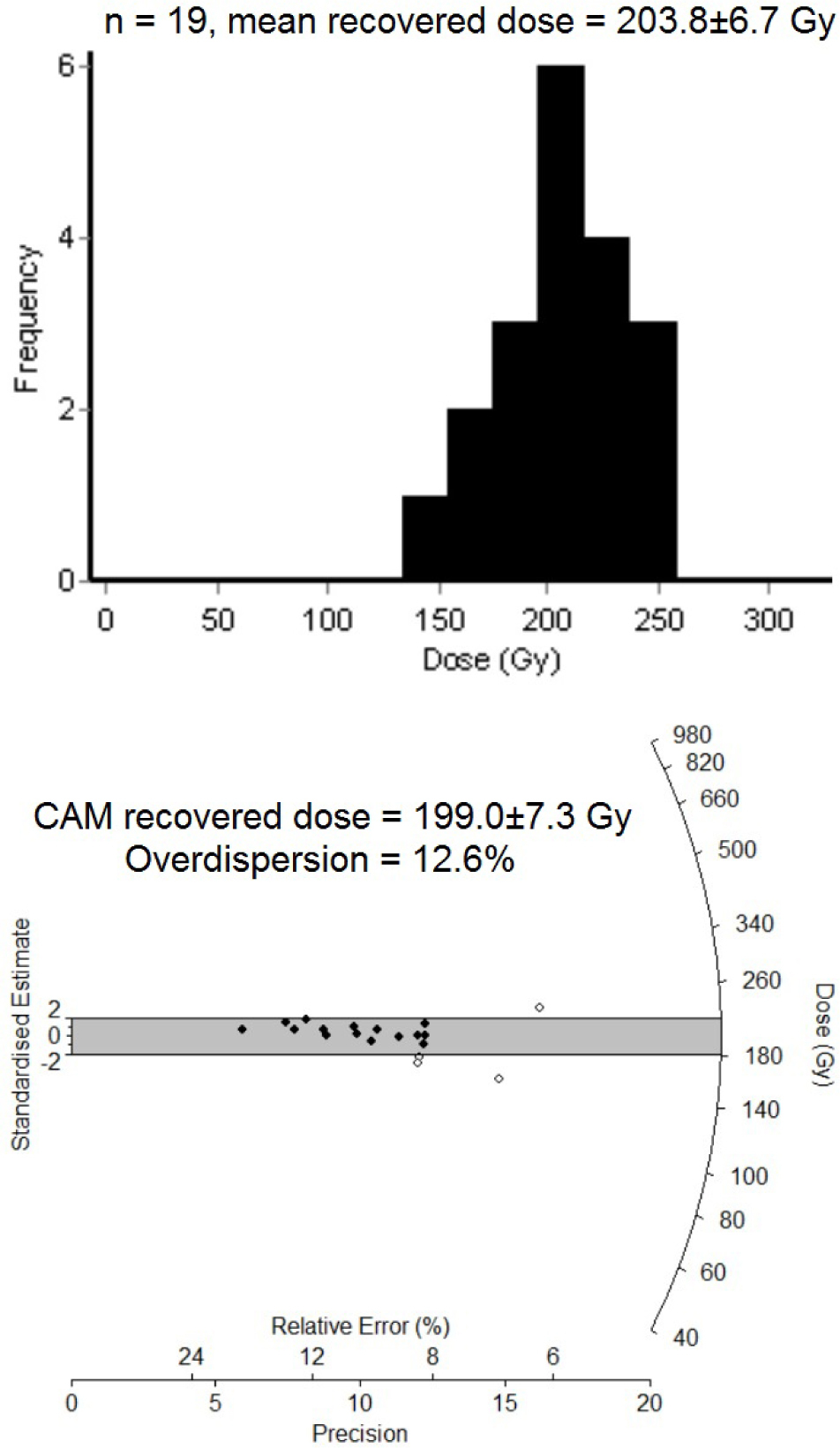
A preheat plateau test was conducted on the sample MN15–1-2, using preheat temperatures from 200°C to 280°C with increments of 20°C. A De plateau was obtained for preheat temperatures from 220°C to 280°C (Fig. 5). Based on the De plateau, a preheat temperature of 260°C for 10 s and a cut-heat temperature of 220°C were selected, except the sample MN15-1-1 in which the preheat temperature was 220°C and the cut-heat was 180°C to minimize thermal transfer effects in such young samples (Wintle and Murray, 2006). To further test the results, a dose recovery test was conducted on sample MN15-3-1. Twenty-four aliquots of the sample were first bleached by an Oriel solar simulator for 2 h, and were then given laboratory dose of 188 Gy, close to the mean natural De value. Such known dose was then treated as unknown, and the aliquots were measured with the SAR protocol in Table 1. Nineteen aliquots have passed recycling ratio and recuperation test. Their results are shown using histograms and radial plots (Fig. 6). The mean and central recovered De values are 203.8 ± 6.7 and 199.0 ± 7.3 Gy respectively, with a small overdispersion of 12.6%. The mean and central dose recovery ratios are thus 1.08 ± 0.04 and 1.06 ± 0.04 respectively, lying within the range of 1.0 ± 0.1. This confirms the reliability of the De measurement results.
Fig. 5
Preheat plateau test for sample MN15-1-2, with a De plateau obtained for preheat temperatures from 220°C to 280°C.
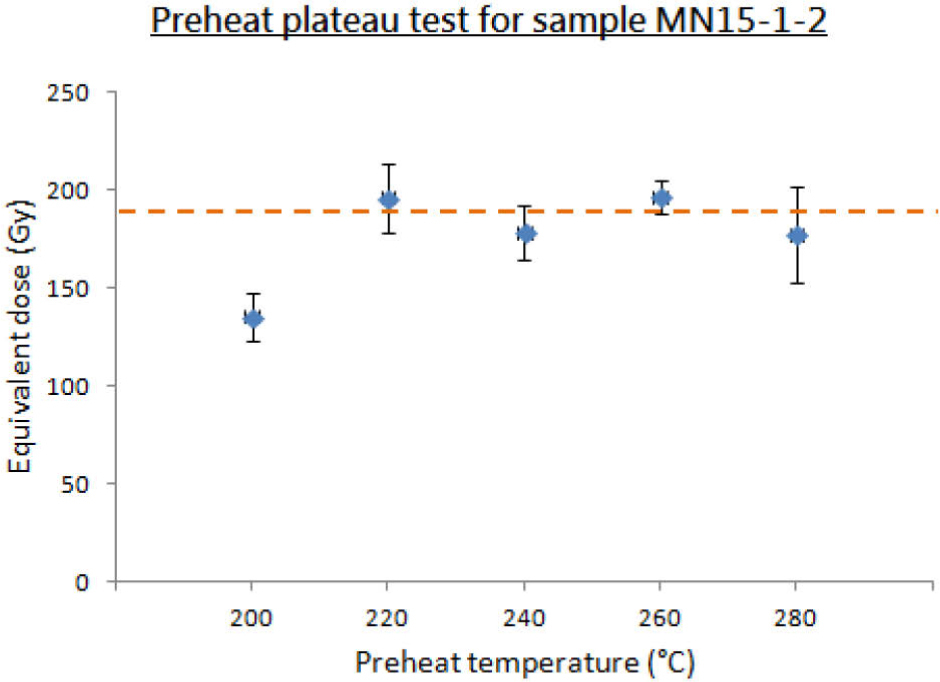
Fig. 6
The distribution of recovered dose values in a dose recovery test of the sample MN15-3-1 is shown using histogram and radial plot. The given laboratory dose was 188 Gy.
For environmental dose rates, the contribution from U and Th decay chains was determined using a Littlemore 7286 thick source alpha counting system, while the contribution from 40K was evaluated by measuring the K content using X-ray fluorescence (XRF). The measured alpha count rate and K content can be converted to dose rates using conversion factors from Adamiec and Aitken (1998). Attenuation of beta dose was calculated using the beta dose absorption fractions reported by Fain et al. (1999) for spherical grains of different sizes. To evaluate the water attenuation effect on dose rate, water content was obtained by weighing the raw samples and dried samples. For samples collected in stainless steel tubes, the ratios of water to the dried mass were used as the water contents. For the block samples, estimated water contents were used (see below), because the blocks have been exposed to air and become almost completely dried. Lastly, the contribution from cosmic ray was calculated from sample’s location, altitude and depth, following Prescott and Hutton (1994).
. OSL dating results
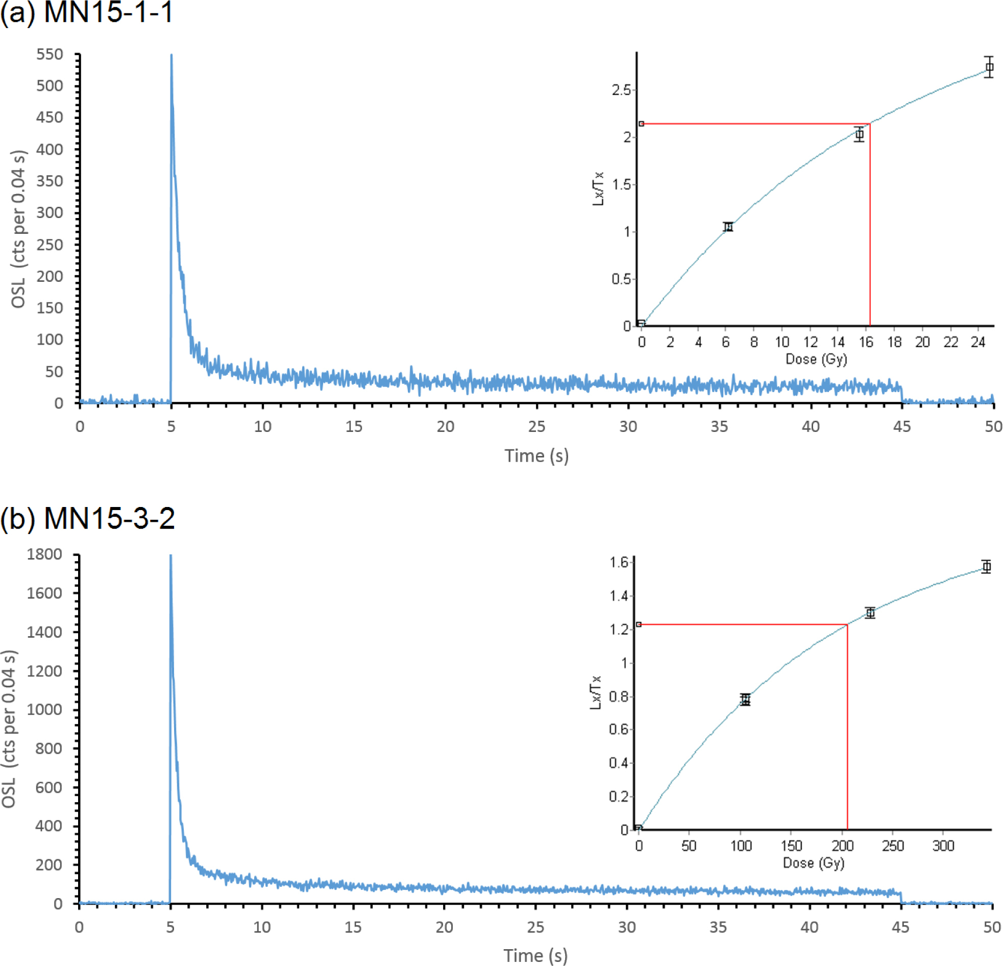
Typical OSL decay curves and dose response curves from samples MN15-1-1 and MN15-3-2 are shown in Fig. 7. The OSL decay curves show rapid decay in the OSL signals, suggesting that the signals are dominated by the fast component. The fast component has been considered to be the most reliable signal for OSL dating (Wintle and Murray, 2006). The influence of medium and slow components was tested by altering the stimulation time integrals used for calculating Lx and Tx. It was found that there was no obvious De dependence on stimulation time for all samples. When an “early background subtraction” method is used instead, more than 80% of aliquots give consistent individual De values with those calculated by “late background subtraction” as described in the procedures above. Also, no systematic differences in the mean and central De are found between both methods, but the “early background subtraction” leads to a larger error due to subtraction of a stronger signal. Thus, subtraction of late background signals from the last 5 s of OSL decay curves were used to calculate the De in the following.
Fig. 7
Typical OSL decay curves and dose response curves (insets) from samples MN15-1-1 and MN15-3-2.
De distributions
De distributions of all the five samples were analyzed using histograms and radial plots (Fig. 8). The arithmetic mean De values, the De derived from central age model (CAM) of Galbraith et al. (1999) and the overdispersion values for the samples are shown in Table 2. Except for MN15-1-1, all samples give overdispersion values of less than 40%. Samples MN15-1-2 and MN15-1-3 have relatively lower overdispersion values of 22.5 and 22.2%, respectively. The radial plots of these two samples (Fig. 8b and 8c) show that most aliquots have De values within 2σ from the central values. Normal distributions can be observed from the De histograms of these two samples. For samples MN15-3-1 and MN15-3-2, they give wider scatters in De values (Fig. 8d and 8e) and higher overdispersion values. However, with the exception of a few poorly bleached aliquots with very large De values, the De histograms of these two samples show a roughly normal distribution.
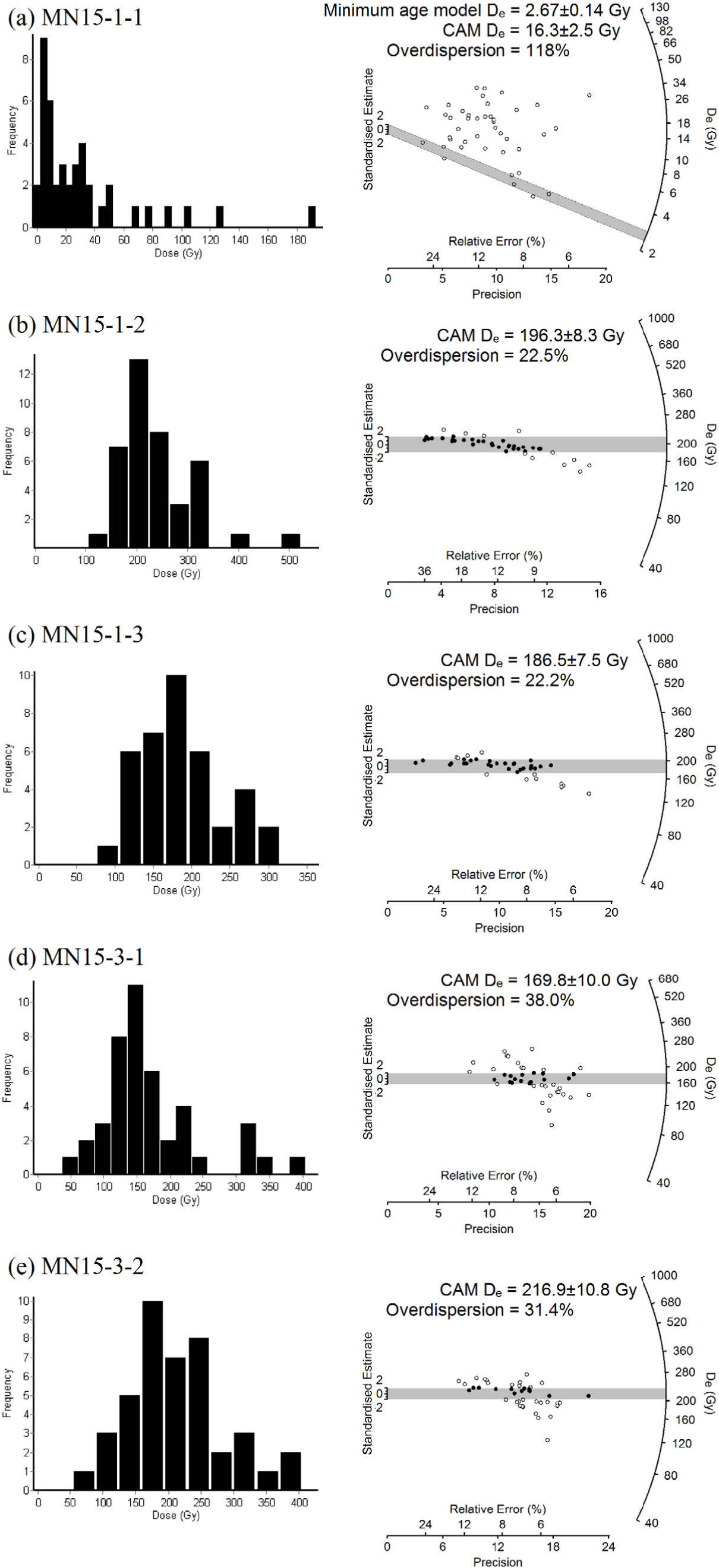
Table 2
The equivalent doses derived from the mean age model and the central age model, with the overdispersion values for the five samples.
| Sample ID | Number of aliquotsb | Mean age model De (Gy) | Central age model De (Gy) | Over-dispersion(%) |
|---|---|---|---|---|
| MN15-1-1 a | 42 | 31.1 ± 5.9 | 16.3 ± 2.5 | 118 |
| MN15-1-2 | 40 | 219.8 ± 11.7 | 196.3 ± 8.3 | 22.5 |
| MN15-1-3 | 38 | 199.7 ± 8.6 | 186.5 ± 7.5 | 22.2 |
| MN15-3-1 | 43 | 183.9 ± 11.7 | 169.8 ± 10.0 | 38.0 |
| MN15-3-2 | 42 | 229.5 ± 11.2 | 216.9 ± 10.8 | 31.4 |
b 48 aliquots were measured for each sample. Aliquots were rejected by various reasons, including failure in recycling ratio test (4, 4, 4, 2, 2) or recuperation test (2, 1, 1, 1, 0), failure in fitting the dose response curve (0, 0, 0, 0, 2) and when the natural Lx/Tx cannot be interpolated onto the dose response curve (0, 3, 5, 2, 2). The five numbers in brackets refer to the number of aliquots rejected by that specific criteria for the five samples (MN15-1-1, 1-2, 1-3, 3-1, 3-2) respectively.
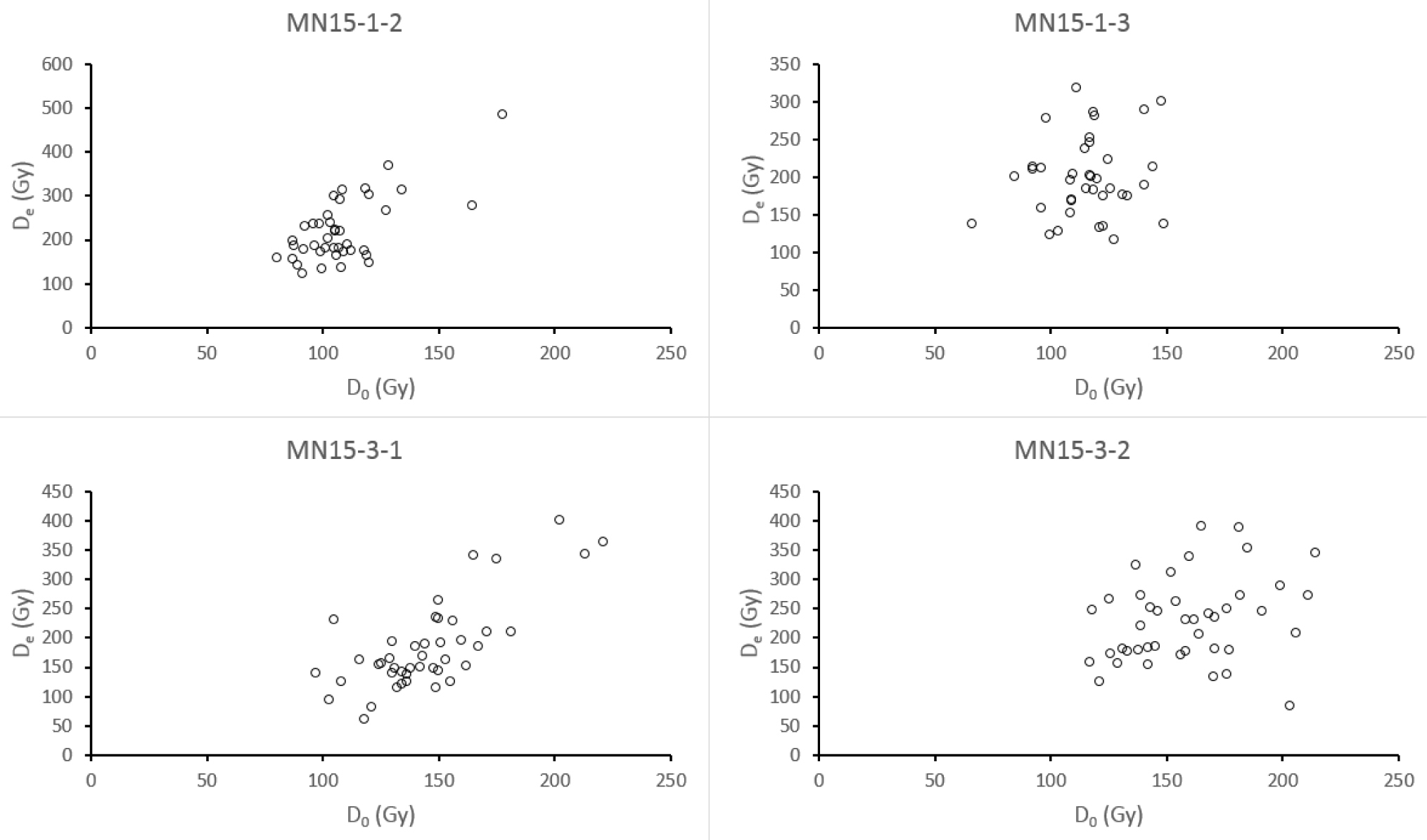
It is noticed that these four samples have relatively high De values close to 200 Gy. Thus, the “2D0” values were also considered. D0 is a constant related to the shape of a dose response curve which can be described by a single saturated exponential of the form Lx/Tx = (Lx/Tx)0[1-exp(−D/D0)]. If De exceeds 2D0, then the result may not be reliable. For our four old samples, the average D0 values for individual samples vary between 112 and 159 Gy. None of the mean nor CAM De values reported in Table 2 exceeded the average 2D0 values, although a small portion of individual aliquots have De > 2D0. The possible dependence of De on D0 for individual aliquots was also investigated (Fig. 9). It was observed that there are no or little dependence of De on D0. Thus, the results can still be regarded as reliable despite larger uncertainties. For these four samples, their arithmetic mean De values are about 10 to 20 Gy larger than the CAM De values (Table 2), but they are consistent with each other within 2σ. Since the mean age model does not consider the errors of individual aliquots, it will give an upward bias if the few aliquots with large De (which have larger errors due to near saturation) are treated equally with the other aliquots. Thus, the CAM De will be used in the following discussion, except the sample MN15-1-1.
Fig. 9
Plots of De vs D0 for individual aliquots of samples MN15-1-2, MN15-1-3, MN15-3-1 and MN15-3-2.
For sample MN15-1-1, the extremely large scatter of De values (Fig. 8a) and an overdispersion of 118% indicates that the sample was insufficiently bleached before deposition. This is in contrast to Wang’s (2014) paleoshoreline sample MS-2B, which was well bleached with a mean natural De of 0.9 Gy and all aliquots give individual De values between 0.8 and 1.1 Gy. This shows that bleaching by sunlight was heterogeneous, even though the samples are from the similar paleoshoreline layer (Figs. 2 and 10). Due to insufficient bleaching problem, the minimum age model (Galbraith et al., 1999; Galbraith and Roberts, 2012) was applied to the sample MN15-1-1. An expected overdispersion of 20% for a well-bleached sample was used in the calculation, based on previously reported values for well bleached sedimentary quartz (Arnold and Roberts, 2009). The natural De obtained for this sample was 2.67 ± 0.14 Gy.
Dose rate evaluation
A summary of the dose rate measurements for different samples are shown in Table 3. The major difficulties in estimating the dose rates come from uncertainties in the water content variation in the past. For site 1, the as found sample water content was assumed in the dose rate calculations, with a relative error of 20%. However, for site 3, the sedimentary section has been exposed for a long time before sample collection, losing most of the moisture content. As the samples from this site were deposited in a lacustrine environment, they must have been under water for a considerable amount of time. Thus, the water content for samples at site 3 was assumed to be 25 ± 5%, which is close to the saturation water content of ~30% estimated in the laboratory. The final calculated dose rates, together with the OSL ages of the samples, are shown in Table 3.
Table 3
OSL dating results for the five samples in the study area.
| Sampling site | Sample ID | Grain size (µm) | Depth (cm) | α-count rate (cts/ks)a | K content (%)b | Water content (%)c | Cosmic ray (Gy/ka)d | Dose rate (Gy/ka) | Equivalent dose (Gy)e | OSL age (ka)e |
|---|---|---|---|---|---|---|---|---|---|---|
| Site 1 | MN15-1-1 | 180–212 | 22 | 4.97 ± 0.12 | 1.48 | 0.12 | 0.21 | 2.36 ± 0.11 | 2.67 ± 0.14 | 1.13 ± 0.08 |
| MN15-1-2 | 150–180 | 50 | 3.12 ± 0.10 | 1.64 | 1.9 | 0.20 | 2.22 ± 0.13 | 196.3 ± 8.3 | 88.5 ± 6.3 | |
| MN15-1-3 | 150–180 | 70 | 2.82 ± 0.09 | 2.03 | 10.6 | 0.20 | 2.32 ± 0.15 | 186.5 ± 7.5 | 80.3 ± 6.0 | |
| Site 3 | MN15-3-1 | 150–180 | 30 | 4.09 ± 0.12 | 2.20 | 25 | 0.21 | 2.32 ± 0.15 | 169.8 ± 10.0 | 73.3 ± 6.4 |
| MN15-3-2 | 125–150 | 90 | 7.71 ± 0.17 | 2.17 | 25 | 0.19 | 2.71 ± 0.16 | 216.9 ± 10.8 | 80.2 ± 6.1 |
. Discussion
Stratigraphic chronology
Site 1
The upper layer of medium to coarse sand with gravels yielded an OSL age of ~1.1 ka (sample MN15-1-1). This age is older than that dated by Wang (2014) from a section along the same paleoshoreline, in which his sample MS-2B (see Figs. 2 and 10) was dated to be ~0.3 ka, corresponding to Little Ice Age. It is noted that this sample is poorly bleached, in contrast to the well-bleached sample of Wang (2014). This means that even aliquots with small De would contain a mixture with a small amount of poorly bleached grains. Thus, the minimum age model would still give an overestimation of ages for MN15-1-1. It may be treated as the maximum age. There may also be uncertainties in dose rate due to heterogeneity of this layer. The exact age of this layer is beyond the scope of the following discussion.
The lower two samples MN15-1-2 and MN15-1-3 give OSL ages of 88.5 ± 6.3 and 80.3 ± 6.0 ka respectively. Although a slight reversal in ages was found, these two ages are consistent with each other within errors. It is noted that the sample MN15-1-3 is mixed with some pebbles which may have different radioactive contents from their surrounding sandy matrix. This potentially gives a large error in the estimation of dose rate. However, based on the ages of these two samples, it is suggested that during ~90–80 ka ago, site 1 was in a paleoshoreline or a near-shore environment, as indicated by the relatively coarse grain sizes of sand. At that time, the paleo-lake level fluctuated at around this site (~262 m a.s.l.). At a certain time after ~80 ka, the lake level retreated. Between ~80 ka and the last ~1 ka, there were no sedimentary records at this site. It is interpreted that a large scale erosion may have occurred in the area. Even if there were lacustrine episodes during this period, the deposited lacustrine sediments would have been eroded away when they were exposed during low lake stands. The eroded materials were likely transported to the adjacent Gurbantunggut Desert by the Westerlies.
Site 3
At site 3, the two lacustrine sand samples yielded consistent OSL ages of 73.3 ± 6.4 and 80.2 ± 6.1 ka respectively. Based on the sedimentary properties and the OSL ages, we deduced that there was a fluvial episode before ~80 ka ago at this site, depositing > 2 m thick layer of greyish gravels. Around 80 ka ago, the lake level of Manas Lake rose and reached above site 3. As a result, fine sand layers were deposited during 80–70 ka ago. But it was interrupted by a brownish mud layer in between. The mud layer could indicate a deeper lake environment. Alternatively, it could be a very shallow lake and calm environment with limited water flow, because the brownish color probably indicates can oxidizing environment. Regardless of how the brownish mud layer formed, it can still be interpreted that the lake level was generally high during 80–70 ka ago. After that, the lake level retreated, with another fluvial episode recorded at the site.
It is not known how long the lacustrine episode has lasted for at this site around 80–70 ka ago, due to the errors of the OSL ages and possible phases of erosion. However, the ages are consistent with that of Fan et al. (2012), who found that there was a stage of high lake stand before ~66 ka at site A (~264 m a.s.l.), which can be associated with a relatively warm and wet climate during late MIS 5.
Paleoenvironmental and neotectonic implications
The results from this study, as well as those of Fan et al. (2012) and Wang (2014), suggest that sedimentary age gap before 1 ka is quite common in the Manas Lake area at an elevation > 260 m a.s.l. At site 1 in this study, a nearly 80-ka sedimentary record is missing in the section. At site A of Fan et al. (2012), there were no records of lacustrine deposition during ~64–48 ka ago and from ~27 ka ago to the present. Also, no young lacustrine sediments (from the Last Glacial Maximum to the present) were found from other sites of Fan et al. (2012), except the lake center which yielded sediments of the last 1 ka. At higher elevations, young sediments were found only in the paleoshorelines, which were also formed within the last 1 ka (Wang, 2014). The age gaps before 1 ka suggest that widespread erosion has occurred in the area. Even if there had been several high lake stands depositing lacustrine sediments, the records would have been eroded away by winds during low lake stands. The last time when massive erosion occurred was probably in an arid climate during 3.6–2.5 ka ago, when increasing aeolian activities were recorded in both the Manas Lake area (Fan et al., 2012) and the adjacent Gurbantunggut Desert to the east (Li and Fan, 2011).
Sites 1 and A currently have similar elevations but are on the opposite side of each other. When the sedimentary sections of the two sites are compared with each other, it can be noted that the sizes of the age gap are different (Fig. 10). A few lacustrine episodes were recorded at site A in the northwestern side of the lake from before 66 ka ago to ~27 ka ago (Fan et al., 2012). However, they were not recorded at site 1 in the southeastern side, despite having a similar elevation. Also, the lacustrine episode at ~73 ka at a higher elevation at site 3 (~8 m higher) on northwestern side was not recorded at site 1. There are two possibilities regarding the difference in age between the sections on the opposite sides of the lake. One possibility is that there has been no differential uplift between site A and site 1 since at least ~73 ka ago. In this case, lacustrine sediments probably once deposited at site 1 during ~73–27 ka ago, but site 1 suffered more erosion and these records were eroded away. However, if paleoenvironments at sites 1 and A were similar during ~73–27 ka ago, then some of the coarser sediments with gravels may also have deposited in site 1, which are more difficult to be eroded away. Such gravel-rich layer is not found in site 1. It is also difficult to explain the differences in erosional rate between the two sites, with the same prevailing westerlies blowing over the largely flat lake area when exposed. Another possibility is that there was a small amount of uplift on the northwestern side of the lake relative to the southeastern side. This case suggests that site A was at a lower elevation (or site 1 was at a higher elevation) than the present. When lacustrine episodes occur, site A was at a more offshore environment than site 1, with more lacustrine sediments deposited. Thus, some lacustrine sediments deposited during ~70–27 ka ago were still preserved at site A of Fan et al. (2012) even after subsequent erosion. This is consistent with previous findings that neotectonics have affected the Manas Lake evolution (Wang, 1991; Mu et al., 2001; Shi et al., 2008; Yao and Li, 2010). Uplift can also explain why there was a shallow lacustrine environment at site 3 (higher elevation in northwestern side) during ~80 ka ago while a paleoshoreline or near-shore environment at site 1 (lower elevation in southeastern side) at about the same time, but such interpretation is limited by the errors in OSL ages.
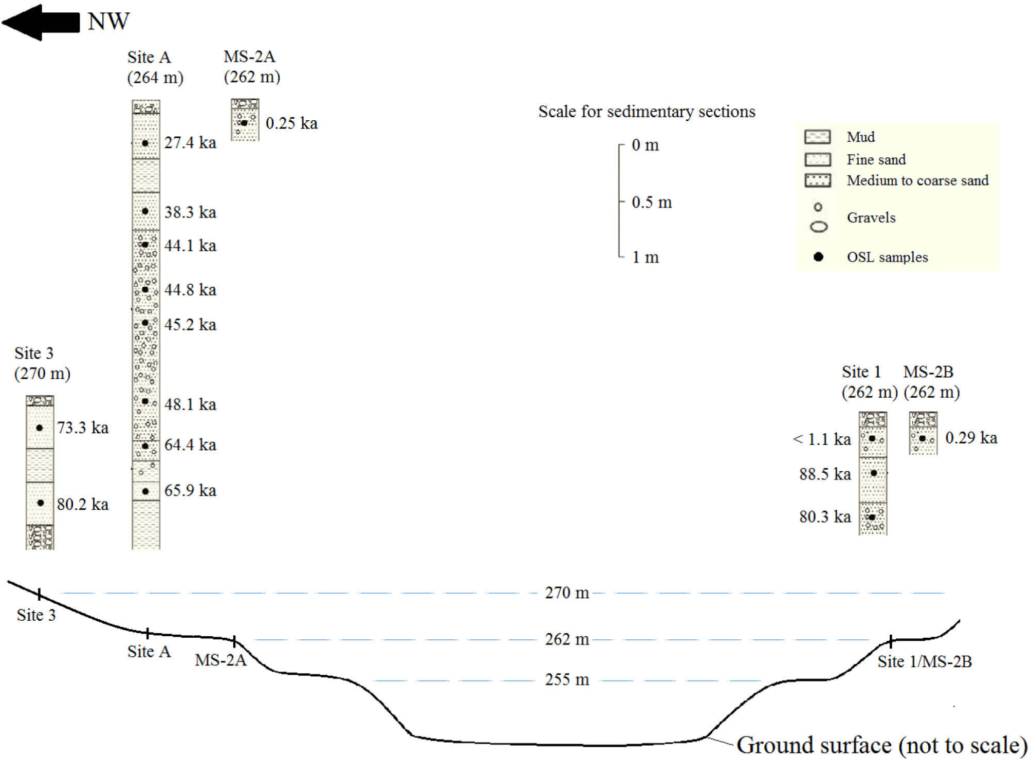
Fig. 10
Summary of results from this studies (sites 1 and 3) and previous studies by Fan et al. (2012) and Wang (2014). Note that the top of each sedimentary section shown corresponds to the ground surface.
. Conclusion
Lacustrine sediments from the northwestern and southeastern sides of Manas Lake were used to study the paleoenvironmental and neotectonic changes in the area, with an OSL chronology established. On the northwestern side of the lake, site 3 (270 m a.s.l.) recorded lacustrine episodes at around 80–70 ka ago. On the other side of the lake, site 1 (262 m a.s.l.) recorded a paleoshoreline to near-shore environment at ~80–90 ka ago, followed by a sedimentary age gap between ~80 ka ago and the last ~1 ka. Combining with the results with those from previous studies (see Fig. 10), it is concluded that breaks in the sedimentary records are common in the area at an elevation of > 260 m a.s.l. Large scale aeolian erosion likely occurred in the area during periods of low lake stands. Furthermore, by comparing sedimentary environments at different times from opposite sides of Manas Lake, it is suggested that a small amount of uplift of the northwestern side relative to the southeastern side of the lake have occurred in the last ~80 ka. Uncertainties still exist in the amount, timing and the spatial extent of the uplift. Future studies may aim to look for lacustrine sediments aged at ~73–27 ka in the southeastern side of the lake, in order to further constrain the paleoenvironment on that side and the extent of differential uplift.