
. Introduction
Over the last decades, luminescence dating of sediments has been established as an indispensable tool in Quaternary research (e.g. Rittenour, 2018). This is in particular due to several methodological developments that have improved over the years the reliability, expanded the dating range and introduced new materials and concepts. Most of these developments such as the single-aliquot regenerative dose (SAR) protocol (Murray and Wintle, 2000), post-IR infrared stimulated luminescence (IRSL) (Buylaert et al., 2009) and the concept of standardised growth curves (Burbidge et al., 2006) focus on the determination of the dose absorbed (palaeodose or equivalent dose, De) since the event that had reset the latent luminescence signal in the mineral grains. However, while reliable determination of the dose rate (Ḋ) is of equal importance for dating, less attention has been paid towards this parameter in recent years. During the last decade, studies mainly focussed, for example, on radiation heterogeneity that adversely affects a desired luminescence age (cf. Guérin, 2018) and on the concentration of dose rate-relevant elements in alkali-feldspar grains (e.g. Smedley and Pearce, 2016). Indeed, in many circumstances, determination of dose rate is straightforward and can be carried out rather routinely. However, there are four main issues with dose rate determination that attracted relatively little attention in the past as these are only relevant under certain circumstances.
First and of ubiquitous importance, it has to be highlighted that the determination of dose rate-relevant elements (K, Th, U) is not without problems. In a comparative study, it was the dose rate that showed large differences between different luminescence laboratories (Murray et al., 2015). As a matter of fact, this is not limited to luminescence dating but also occurs in proficiency tests of geo-analytical laboratories, for example, for a loess from Nussloch (GeoPT13; Potts et al., 2003; IAG, 2022), a typical sediment dated by luminescence. Hence, crosschecking the performance of the measurement procedures with certified reference material (CRM) or by comparing different analytical approaches is highly advisable. Second, the average moisture content of a sample since the event to be dated plays an important role as pore water has an attenuation effect on ionising radiation (Zimmerman, 1971), which affects dose rate determination (Nathan and Mauz, 2008). For calculation of a correct age, the estimation of an appropriate long-term average water content is important. However, the modern water content of a sample does not necessarily reflect the average sediment moisture during burial (e.g. Nelson and Rittenour, 2015). Furthermore, some sediments such as lake deposits experience compaction with time, hence a significant change in pore space and water content (e.g. Juschus et al., 2007; Lukas et al., 2012). While several procedures allow to determine the maximum water uptake capability, in most of these, the structure of the sediment is destroyed, and the effect of compaction on pore space is lost (Lowick and Preusser, 2009). Third, the common assumption in luminescence dating is that the sample is taken from an infinite homogenous layer with regard to radiation from radioactive decay. This is applicable as long as the material 30 cm around the sample can be regarded homogenous, but this may not apply in all settings (Brennan et al., 1997; Degering and Degering, 2020). Fourth, a basic assumption is that the dose rate remains constant with time, but besides changes in water content and sediment overburden (which affects the cosmic dose rate), some samples are affected by radioactive disequilibrium. The latter describes the loss or gain of radionuclides from the uranium decay chain (e.g. Krbetschek et al., 1994; Prescott and Hutton, 1995; Olley et al., 1996; Guibert et al., 2009). Examples are an initial surplus of U-238 compared to its daughter isotopes in samples rich in shell material (Zander et al., 2007) or the uptake of U-238 by organic-rich (peaty) material from percolating ground water (Preusser and Degering, 2007). Identifying such disequilibria is most effectively done using high-resolution gamma spectrometry (HR-GS) that allows for the measurement of different nuclides from the decay chain.
Presented here is a dating application that addresses all four aforementioned issues related to dose rate determination. The material investigated is from two scientific drill cores in the village of Niederweningen in northern Switzerland that is known for the Pleistocene fauna that has been discovered there, in particular the remains of several individuals of mammoth, and related environmental reconstructions (Furrer et al., 2007). The coring targeted lacustrine and palustrine deposits that presumably formed during the early Late Pleistocene. These sediments are partly rich in organics (peat), which previously have proven problematic concerning water content assessment and radioactive disequilibria (Preusser and Degering, 2007). The sequence is furthermore in some parts characterised by thin layers, and it was considered prudent to crosscheck the performance of gamma spectrometry with an independent approach, in this case neutron activation analyses (NAA). Besides the relevance for this particular site, the study exemplifies potential pitfalls, solutions and limitations when dating similar sediment sequences. To illustrate the effects of different correction steps (i.e. water content, layer modelling and radioactive disequilibrium), these are subsequently carried out individually and evaluated, before finale age estimates are discussed.
. Regional Setting and Study Site
Niederweningen is located in the overdeepened trough of Wehntal, a 5-km-long east-west orientated valley in the northern Alpine foreland of Switzerland (Fig. 1A). The eastern entrance of the valley is characterised by a terminal moraine ridge, which formed by a lateral lobe of the Walensee Glacier during the maximum extent of the Last Glaciation (Preusser et al., 2011). At the western end of the valley, the small stream of the Surb is cutting into molasse hills, resulting in a gorge-like valley shape. To the south, the valley is bordered by the Lägern anticline structures, which is composed of Jurassic carbonates, while the northern slope of the valley comprises molasse bedrock covered by Early Pleistocene ‘Deckenschotter’ gravel deposits (Graf, 1993).
Fig 1.
(A) – Map indicating the location of the study area in the Swiss Alpine foreland with the extent of the LGM ice cover (blue-green) and overdeepened structures below the present day land surface (grey). (B) – Detailed map of the Wehntal with the location of previous (white circles) and present (black circles) sites investigated in the village of Niederweningen (modified after Dehnert et al., 2012). LGM, last glaciation maximum.
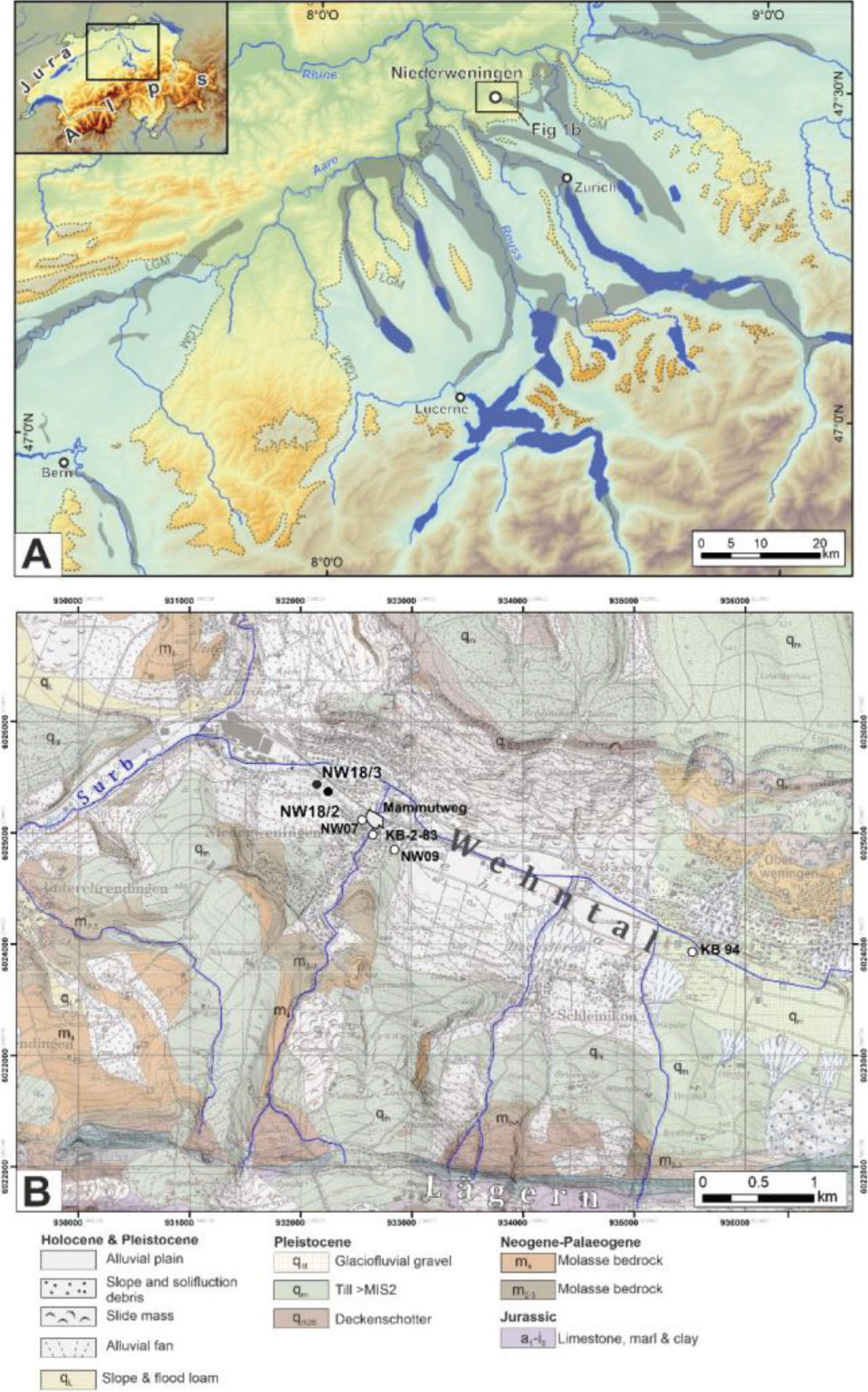
Previous research has focussed on sites located a few 100 m apart from the sites analysed here (Fig. 1B; core KB 2-83, Welten, 1988; core NW07, Anselmetti et al., 2010; core NW09, Dehnert et al., 2012; construction pit ‘Mammutweg’, Furrer et al., 2007). According to these studies, the sedimentary succession filling the overdeepened trough of the Wehntal records at least two glacial advances during marine isotope stage (MIS) 6, with the first advance (c. 185 ka) possibly carving out the basin (Dehnert et al., 2012). Following a second glacial advance (c. 140 ka), the valley was covered by a proglacial lake, which gradually silted up during MIS 5 and 4. The shifting of depositional environments to alluvial and fluvial influenced wetlands as well as changes in climate resulted in a complex sedimentary sequence, which includes several peat horizons, in particular a prominent upper and a lower peat unit (Anselmetti et al., 2010; Dehnert et al., 2012). The lower peat unit has previously been suggested to be of late Eemian (MIS 5e) age based on its pollen assemblage (Anselmetti et al., 2010), while the upper peat unit, also called ‘mammoth peat’ due to its rich fossil vertebrate record, has been dated to about c. 45 ka (MIS 3, Hajdas et al., 2007; Preusser and Degering, 2007).
In this study, we illustrate the challenges of dating sediments deposited in such a complex setting with luminescence methods by analysing two drill cores with a diameter of 220 mm, which were recovered during a drilling campaign utilising a rotary drill rig in late 2018. The cores NW2018/2 (16.0 m length) and NW2018/3 (16.7 m length) are located more than 500 m NW of previous coring locations (Fig. 1B) and show a similar sedimentary sequence as described earlier). However, in contrast to previous coring locations, there are not two distinct peat units, but rather a complex sequence of interbedded partly organic-rich silt/sand layers and peat (Fig. 2). Similarly to a previous study (Anselmetti et al., 2010), four main lithotypes (LTs, labelled 1–5) and several distinct subtypes (labelled a–f) can be defined within this sequence based on the dominant grain size, sorting, grain lithologies and organic content.
Fig 2.
Logs of the cores NW2018/2 and NW2018/3 illustrating the LTs, lithology and OSL sample locations as well as the layer model used for the individual OSL samples. LTs, lithotypes; OSL, optically stimulated luminescence.

Within core NW2018/2, the organic-rich sequence spans from 7.62 m to 4.17 m depth and is associated with thin interbedded silts and clays. Beneath 7.10 m, these silts are light grey to green and contain mollusc shells (LT: 3c), while above, the clastics interbedding with the peats are predominantly dark grey, organic-rich silty clays (LT: 2b) or dark brown organic-rich sandy silts (LT: 3d). The organic-rich deposits can be differentiated into dark brown silty gyttia with few plant remains (LT: 1a), compacted dark brown to black muddy-silty peat with few wood fragments (LT: 1b) and dark brown to silty peat many wooden fragments (LT: 1c). Above the organic-rich interval, sandy silts of light grey to dark grey colour and with small plant remains occur (LT: 3f).
Within core NW2018/3, the organic-rich sequence spans from 5.05 m to 2.47 m depth. In contrast to NW2018/02, the interbedded clastic layers are generally of coarser nature, highlighted by the occurrence of a dark grey pebbly silty sand in which plant remains are observed (LT: 4b), and the presence of pebbles within one of the peat layers. Above the peat interval, graded sands with large pebbles occur (LT: 4a).
. Methods
. Sediment Properties
After drilling, the two cores were stored indoors in wooden boxes and were split in half just prior to sampling for luminescence dating. The cut surfaces were carefully prepared and photo-documented prior to further analysis. Following a macroscopical sedimentological description, samples were taken every 10 cm for grain size and compositional analysis. For laser-optical grain size analysis, a first batch of all samples were pre-treated with 20% H2O2 at 70°C for 24 h to degrade organic matter. Thereafter, Calgon (a solution of 33 g sodium hexametaphosphate and 7 g sodium carbonate) was added to the samples, and after a 24-h period, analysis was performed with a Malvern Mastersizer 3000 (Abdulkarim et al., 2021). For a second batch, after oven-drying, the sediment at 105°C for 24 h, organic matter and carbonate content were determined by the loss-on-ignition method using a muffle furnace at a temperature of 550°C for 3 h for organic matter and 950°C for 2 h for the carbonate content (Heiri et al., 2001). In addition, the water absorption capacity of selected sediment samples was determined using the Enslin–Neff method (DIN 18132:2012-04), which analyses the water uptake of 1 g of oven-dried (105°C for 24 h) powdered samples over time using the Enslin–Neff device (cf. Kaufhold and Dohrmann, 2008). The first reading of the burette was recorded after 15 s, following the power law. Repeated measurements were done for each sample to check the reproducibility. For most samples, the water uptake was finished after 4 min, while for organic-rich samples, the procedure took up to 24 h. The sedimentological description and the results of the geochemical and grain size analyses were used here to define LTs occurring in the cores, but their environmental interpretation will be discussed in a separate publication.
. Equivalent Dose Determination
Since the cored sediments were directly transferred to wooden boxes (no use of opaque liners), samples for luminescence dating had to be taken as large pieces of compact material (typically 10–20 cm length in all dimensions; a minimum of 1 kg of material). A first batch of samples was taken few weeks after the drilling operation, when cores were kept in a cool place (sample numbers up to 11). A second batch of samples (sample numbers above 20) was taken more than 1 year after drilling, when sediment in part had substantially dried out. An overview of the location and sedimentary context of the different samples is given in Table 1.
Table 1.
Overview of samples and their sedimentary context.
Under subdued red-light conditions in the laboratory, the outer light-exposed parts of the lumps were first generously removed (>1 cm), gaining some 100 g of sediment that was not exposed to light. The removed sediment was used for dose rate and other analyses. Part of the remaining material (some 10 g) was subsequently treated with 10% HCl, 30% H2O2 and Na-oxalate to remove carbonates and organic material as well as to dissolve clay particles. The fraction 4–11 μm was enriched by settling (Stokes’ law) using a combination of Atterberg cylinders and centrifuging (cf. Frechen et al., 1996). The retrieved material was split, and one part was directly used for measurements (polymineral fraction). The other part was treated for 1 week in 30% H2SiF6, followed by 10% HCL treatment, to dissolve feldspar (quartz fraction). However, only for 10 out of 19 samples, enough material for measurements was gained by this approach. The material was dispersed in water and pipetted on stainless steel discs (ca. 2–3 mg per disc).
The measurement set-up was chosen to be similar (close to identical) to previous studies at this site (Preusser and Degering, 2007; Anselmetti et al., 2010; Dehnert et al., 2012), using modified versions of the SAR protocol of Murray and Wintle (2000). All measurements were done on an upgraded Risø TL-DA-15 reader, equipped with blue and IR diodes. For quartz, optically stimulated luminescence (OSL) of quartz was recorded during a 60-s stimulation at 125°C using a Hoya U-340 detection filter, after pre-heating for 10 s at 230°C. This was identified performance test (dose recovery, thermal transfer, preheat plateau) by Anselmetti et al. (2010). The OSL signal is characterised by rapid decay typical for quartz (Fig. 3A). The first 0.4 s of the OSL readout were used for signal integration with the integral 50–60 s subtracted as background. IRSL of the polymineral fraction (expected to be dominated by feldspar emissions) was stimulated for 60 s at 50°C using the combination of a Schott BG39 and a Corning 7-57 filter. A pre-heat of 270°C for 10 s was applied, following Anselmetti et al. (2010). The first 10 s were used for signal integration, with background subtraction of the last 10 s. For both the quartz and polymineral fraction, a double saturation exponential function was used for fitting dose–response curves. For quartz, five aliquots were measured, all passing the commonly applied rejection criteria (signal three-time above background, recuperation <10% of natural, recycling ratio within 10% of unity, test dose and De error <10%; cf. Wintle and Murray, 2006). For the polymineral fraction, a total of seven aliquots was measured, of which some had to be rejected. The rather low number of replicate measurements compared to coarse-grain (sand) dating is justified as fine-grain discs contain more than a million grains and usually show a very low level of scatter (typically relative standard deviations are around 5%). However, it is also not possible to infer regarding the presence of partial bleaching from inter-aliquot variability of De values.
Fig 3.
Characterisation of luminescence properties exemplified for sample NW19-3-8. Shown are (A) OSL and (B) IRSL decay curves together with the sensitivity change observed during the course of the SAR protocol (plot of Tn/Tx), (C) dose–response curves for both OSL and IRSL, and (D) plot of mean (CAM) OSL versus IRSL De values. IRSL, infrared stimulated luminescence; OSL, optically stimulated luminescence; SAR, single-aliquot regenerative dose; CAM, Central Age Model.
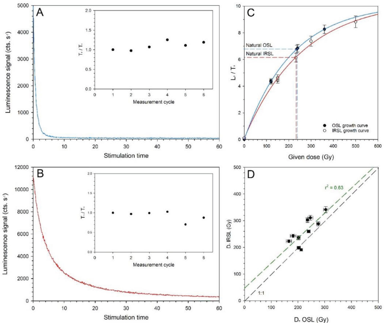
The characteristics of the luminescence behaviour are summarised in Fig. 2. This reveals quite strong OSL (Fig. 3A) and IRSL (Fig. 3B) response with limited sensitivity change. The natural signal for both OSL and IRSL plots on parts of the respective dose–response curve that are far from saturation (Fig. 3C). Nevertheless, there is a clear offset in the De values determined for the two approaches with 8 out of 10 IRSL values plotting above the line of equality (Fig. 3D). This issue will be addressed in the discussion.
. Dose Rate Determination
High-resolution gamma spectrometry at the University of Freiburg was carried out using a high-purity germanium (HPGe) detector (Ortec GMX30P4-PLB-S, n-type coaxial, 30% relative efficiency, 1.9 keV Full Width at Half Maximum at 1.33 MeV). After drying the sample material at 50°C, containers with a diameter of 75 mm and a height of 30 mm were completely filled with homogenised sediment (crushed to <2 mm), sealed with adhesive tape, and stored for at least 4 weeks to build up equilibrium between radon (Rn-222) and its daughters. The sediment mass varied between 75 g and 161 g per sample depending on its density. After storage, the sample containers were placed on the carbon fibre endcap of the detector and were measured for 3 days or 4 days, respectively, to determine the activities of primordial radionuclides K-40, Th-232 and U-238. The detector is installed in a massive lead shielding to minimise the influence of the environmental radioactivity. Additionally, a blank sample (empty container) was measured to account for background radiation.
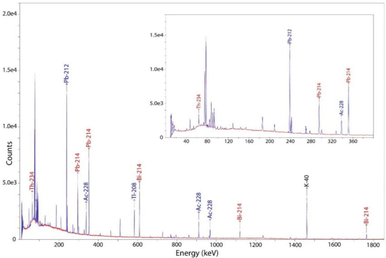
The gamma spectrometer was calibrated using the certified Weichselian loess from Nußloch quarry near Heidelberg, Germany (Koeln Loess, Potts et al., 2003, also known as UoK Loess, IAG, 2022). Repeated measurements of the reference material over several months reveal good reproducibility (Table 2). The gamma spectra (Fig. 4) were analysed using GammaVision 7.01 (Ortec). The U-238 activity was determined by analysing the Th-234 (direct U-238 daughter) line at 63.3 keV. In addition, the peaks of the Ra-226 daughters Pb-214 (295.2 keV and 351.9 keV) and Bi-214 (609.3 keV, 1120.3 keV, 1764.5 keV) were analysed. The comparison of these two values is used to quantify possible radioactive disequilibria in the U-238 decay chain. The Th-232 activity was estimated by analysing the peaks of the Ra-228 daughter Ac-228 (338.3 keV, 911.2 keV, 969.0 keV) and the Th-228 daughters Pb-212 (238.6 keV) and Tl-208 (583.2 keV). K-40 was measured directly at 1460.8 keV. The weighted mean of all selected peaks was calculated to determine the activities of the parent radionuclides U-238 and Th-232, respectively. The uncertainties reflect only the statistic uncertainties of the counting results.
Table 2.
Results of repeated gamma spectrometry measurements of reference material ‘Koeln Loess’ in comparison with NAA and reference values.
| Parent nuclide | Daughter nuclide | Energy (keV) | Meas. 1 12/2019 | Meas. 2 06/2020 | Meas. 3 10/2020 | Meas. 4 4/2021 | NAA | Reference Potts et al. (2003) (IAG, 2022) |
|---|---|---|---|---|---|---|---|---|
| Activity (Bq/kg) | ||||||||
| U-238 | Th-234 | 63.3 | 28.0 ± 1.2 | 35.6 ± 1.4 | 33.9 ± 1.4 | 34.3 ± 1.4 | ||
| Pb-214 | 295.2 | 32.1 ± 0.7 | 34.1 ± 0.7 | 33.8 ± 0.7 | 34.2 ± 0.7 | |||
| Pb-214 | 351.9 | 32.0 ± 0.7 | 33.2 ± 0.7 | 33.6 ± 0.7 | 33.3 ± 0.7 | |||
| Bi-214 | 609.3 | 31.9 ± 0.7 | 33.3 ± 0.7 | 33.5 ± 0.7 | 33.0 ± 0.7 | |||
| Bi-214 | 1120.3 | 29.5 ± 0.6 | 36.5 ± 0.8 | 33.5 ± 0.7 | 35.1 ± 0.7 | |||
| Bi-214 | 1764.5 | 32.8 ± 0.7 | 34.1 ± 0.7 | 33.6 ± 0.7 | 32.7 ± 0.7 | |||
| Mean | 31.6 ± 1.3 | 34.2 ± 1.3 | 33.6 ± 0.1 | 33.6 ± 0.9 | ||||
| Concentration | (ppm) | 2.56 ± 0.10 | 2.77 ± 0.10 | 2.72 ± 0.01 | 2.72 ± 0.08 | 2.49 ± 0.19 | 2.70 ± 0.19 (2.75 ± 0.09) | |
| Th-232 | Ac-228 | 338.3 | 32.4 ± 0.7 | 32.5 ± 0.7 | 34.1 ± 0.8 | 32.0 ± 0.7 | ||
| Ac-228 | 911.1 | 34.0 ± 0.8 | 32.9 ± 0.7 | 32.4 ± 0.7 | 32.7 ± 0.7 | |||
| Ac-228 | 969.1 | 34.2 ± 0.8 | 33.3 ± 0.7 | 31.7 ± 0.7 | 31.7 ± 0.7 | |||
| Pb-212 | 238.6 | 32.1 ± 0.6 | 33.3 ± 0.7 | 33.1 ± 0.7 | 32.8 ± 0.6 | |||
| Tl-208 | 583.2 | 33.3 ± 0.8 | 33.7 ± 0.8 | 33.0 ± 0.7 | 33.6 ± 0.8 | |||
| Mean | 33.1 ± 1.0 | 33.1 ± 0.5 | 32.8 ± 1.8 | 32.5 ± 0.7 | ||||
| Concentration | (ppm) | 8.16 ± 0.24 | 8.16 ± 0.12 | 8.10 ± 0.45 | 8.02 ± 0.17 | 7.68 ± 0.39 | 8.11 ± 0.47 (8.27 ± 0.21) | |
| K-40 | - | 1460.8 | 339.1 ± 7.0 | 336.5 ± 6.8 | 335.0 ± 6.8 | 335.6 ± 6.8 | ||
| Concentration | (%) | 1.10 ± 0.02 | 1.09 ± 0.02 | 1.08 ± 0.02 | 1.09 ± 0.02 | 1.04 ± 0.06 | 1.08 ± 0.02 (1.11 ± 0.01) | |
[ii] The spectrometer used was calibrated against values given in Potts et al. (2003).
[iii] Conversion of activity into concentrations follows Guérin et al. (2011).
Fig 4.
Gamma ray spectrum of the reference loess material (Koeln Loess). Sample weight: 160.5 g, measurement time: 584,786 s. Selected peaks are labelled with the corresponding nuclide names, red: U-238 daughter nuclides, blue: Th-232 daughter nuclides. The inset focusses on the lower energy range of the spectrum from 0 keV to 400 keV.
Additional long time measurements on selected samples were performed by VKTA – Radiation Protection, Analytics & Disposal, Rossendorf in the underground laboratory ‘Felsenkeller’ (Niese et al., 1998) to determine the weak gamma emission of Th-230. The gamma spectrometers contained HPGe detectors of 30% … 90% relative efficiency and are especially designed for low-level applications.
Multi-element NAA analyses (cf. Laul, 1979; Greenberg et al., 2011) were carried out by Bureau Vertias, Canada. The procedures applied (Bureau Vertias, 2019) include that samples are irradiated at the McMaster Nuclear Reactor, where they are exposed to a neutron flux. Nuclear reactions such as neutron capture result in the formation of unstable nuclei, which are identified and quantified by their gamma emissions. Element contents are calculated by referring to standard materials and applying corrections for the actual flux using flux monitors. NAA allows direct determination of 238U, the mother isotope of the uranium decay chain that is in particular affected by radioactive disequilibrium. Dose rates and ages were calculated using ADELE-2017 software (https://add-ideas.com; Degering and Degering, 2020). Following Anselmetti et al. (2010), a-values of 0.07 ± 0.02 (polymineral) and 0.04 ± 0.01 (quartz) were used. The cosmic dose rate was corrected for depth and geographical position following Prescott and Hutton (1994).
. Addressing the Different Dosimetric Issues
. Comparison of Gamma Spectrometry with NAA Analyses
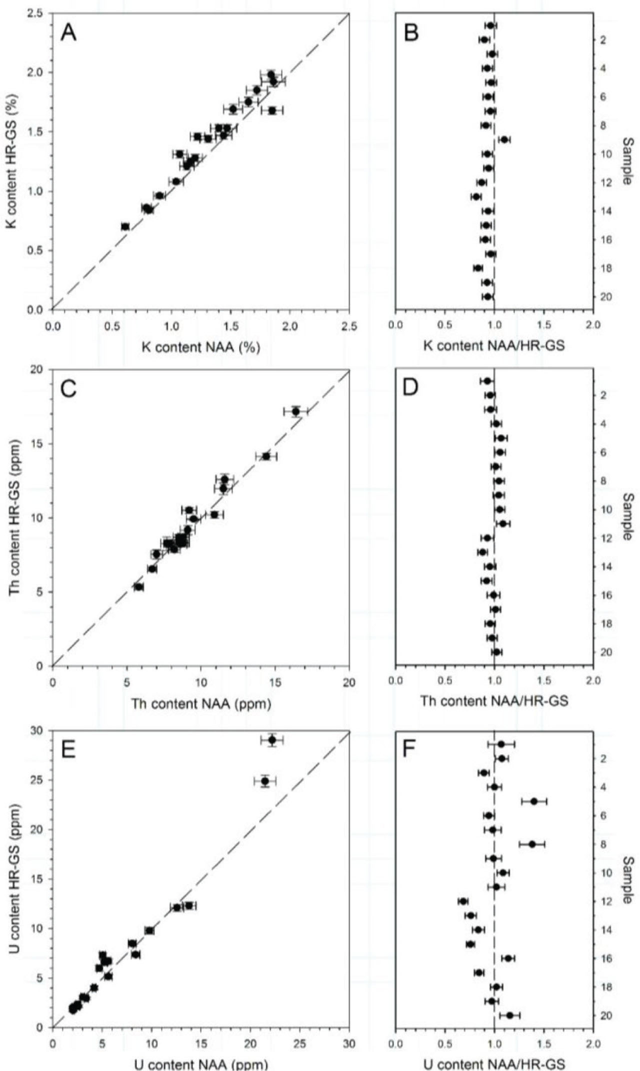
The measured concentration of dose rate-relevant elements and radionuclides is given in Table 3 and plotted in Fig. 5, showing both absolute values as well as ratios. For potassium, a slight but systematic offset between the two methods is observed, with only one sample showing a higher NAA value than gamma spectrometry. The average ratio of NAA/gamma spec is 0.93 ± 0.06, which indicates that the NAA values are, on average, 7% lower. However, both NAA and gamma spectrometry recover the K-value of the CRM within uncertainties, which does not permit to favour one of the approaches as being more accurate. For thorium (Th-232), all but two values plot on the line of equality within uncertainties (1δ), with an overall ratio of 0.99 ± 0.06. For uranium (U-238), the average value of 1.00 ± 0.19 reveals an overall good match but with a high degree of variability. It should be noted that the determination of U-238 is based on the analysis of a low energy gamma line (63.3 keV) of its daughter Th-234. The low gamma energy results in an enhanced sensitivity of the analysis to self-absorption effects, caused by differences in matrix composition and bulk density between the measured sample and the CRM. Peaks of higher energies (>100 keV) like those of the radon successors Pb/Bi-214 could not be used for this comparison because of the occurrence of U-238/Ra-226 disequilibria. The largest offset is observed for the two highest absolute values determined for samples NW18/2-23 and NW18/2-24. These two samples are from organic-rich deposits, and their composition has the largest deviation from that of the loess CRM.
Table 3.
Concentration of dose rate-relevant elements (K, Th, U) determined by both NAA and HR-GS.
[ii] For the latter method, the concentration of U-238 and Ra-226 (average of all post-radon isotopes) is given.
[iii] The ratio of the two values indicates surplus (if >1.00) or deficit (if <1.00) of nuclides from the early part of the decay chain.
[iv] The implications of such radioactive disequilibria are discussed in Section 4.4.
. Sediment Moisture
For a realistic assessment of the water content, the sediment moisture at the time of sampling as well as the water absorption capacity of each sample were determined (Fig. 6). The water absorption capacity determined by the Enslin–Neff experiment is for all samples higher than the sediment moisture measured after core sampling, on average, by 26%. This is expected as the cores were stored for several weeks before sampling was carried out, and thus, the sediment had partly dried out. Additionally, the Enslin–Neff experiment gives the maximum water absorption capacity of loose (disintegrated) sediment, which is likely higher than the water content within a compacted sediment.
Fig 6.
Sediment moisture at the time of sampling plotted versus water absorption capacity. Note that the water absorption capacity of all samples is higher than the sediment moisture. The organic content also influences the water content, with samples with a high organic content featuring higher water contents. Dashed = 1:1 line, dotted line: y = x + 25.
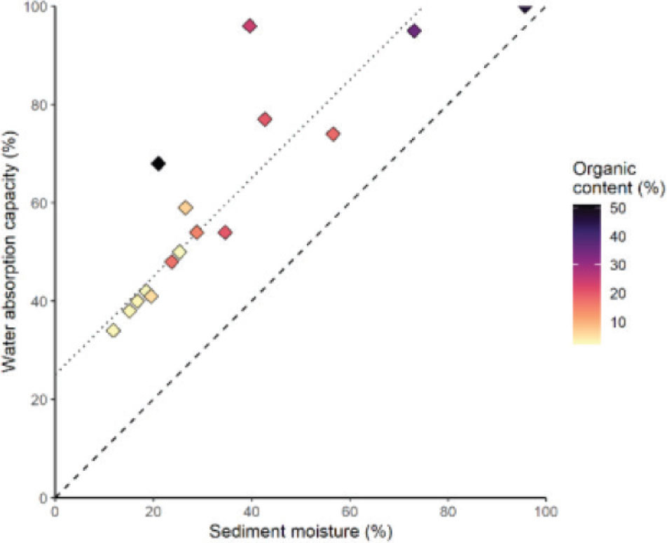
Samples with a high organic content generally have a higher water content than samples with a low organic content; however, even peat samples only show a water absorption capacity of 54%–160% (Table 4). This is in contrast to the literature according to which the natural water content of unconsolidated peat ranges from 200% to 2200% (Huat et al., 2011). This is likely due to the fact that peat commonly does not swell up upon re-saturation, and dried peat is incapable to absorb more than 30%–55% of the original water content. Even if a compaction, and thus reduction of the pore space and water content, of 50% is assumed for the 4–7 m deep buried peat layers, the in situ water content is likely underestimated by at least 25% using Enslin–Neff methodology.
Table 4.
Listing the three different water contents used to test the influence of water content on dose rate calculations.
For the organic-poor silts, the long-term water content is more likely to have between the sediment moisture at the time of sampling and the experimentally determined maximum water absorption capacity. To test the impact of the long-term water content on dose rate and age determination, three different water contents are used: (1) the sediment moisture during sampling; (2) the water adsorption capacity, including a correction for peat-rich samples (adding 25% on top of the observed value); and (3) an estimated long-term water content based on the sediment properties and the water contents calculated by approaches (1) and (2) (Fig. 7).
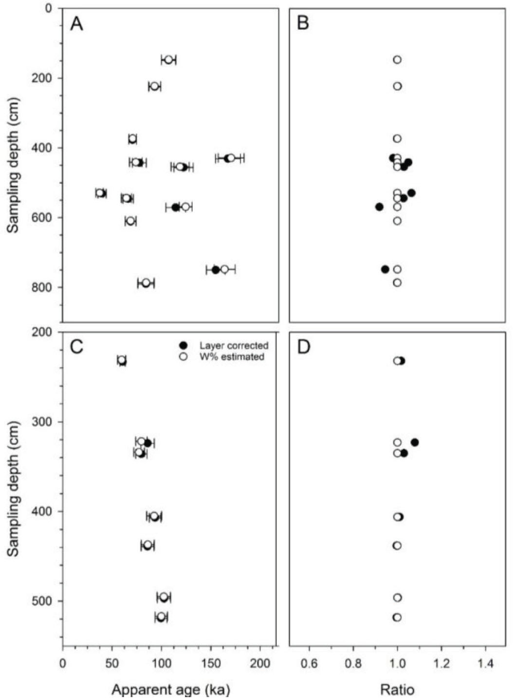
Fig 7.
Illustrating the impact of different water contents on the IRSL ages of core NW18/2 (A,B) and NW18/3 (C,D). A and C show the absolute values, whereas B and D display the ratio in comparison to the estimated water content. Closed circles (scenario 1): sediment moisture determined after sampling. Triangles (scenario 2): maximum water adsorption capacity measured in the laboratory, including adding 25% for peat samples. Open circles (scenario 3): estimated long-term water content based on the sediment properties and the water contents determined by scenarios 1 and 2. Scenario 3 is our preference and is used in the following when applying other correction factors than water content. IRSL, infrared stimulated luminescence.
The effect of applying different sediment moisture scenarios is displayed in Fig. 7, separately for both cores, and shown are both absolute and relative values. Due to the fact that only for part of the samples, quartz OSL ages are available, and to keep the discussion straightforward, the impact of dose rate issues on age is only discussed for polymineral IRSL, and using the results of gamma spectrometry only. Core NW3 shows an increase in the IRSL ages with depth from c. 65 ka to c. 107 ka (Fig. 7C), with age estimates using the measured water content being some 10%–20% lower than those based on the estimated water content (Fig. 7D). A similar range is observed for core NW2 (Fig. 7A), but ages from this core are highly scatter and do not follow stratigraphy (i.e. ages do not systematically increase with depth). For three of these samples (NW18/2-23, NW18/2-07, NW18-2-24), using the measured water content results in about 40% lower ages estimates (Fig. 7B).
. Sediment Layering and Inhomogeneous Radiation Fields
The studied sediment sequence captures a change in the depositional environment from a lacustrine setting to alluvial- and fluvial-influenced wetlands under changing climatic conditions. As a result, the sedimentary sequence comprises interlayered silts, clays and peats, with individual bed thicknesses often less than 30 cm (Fig. 2). While such complex interbedding is common in continental Quaternary records, it poses a challenge for luminescence dating as each of the layers has differing compositions and thus dose rates (Aitken, 1985; Degering and Degering, 2020). The layering will hence cause inhomogeneity in radiation fields but limited to γ-rays, due to the limited range of α- and β-radiation in sediments (c. 20 μm and 2 mm, respectively).
We use a three-layer model to account for the different dose rates that is implemented in ADELE-2017: the sampled layer L, the overlying layer A and the underlying layer B (Fig. 8). Only the sedimentary sequences 30 cm above and below the sampling interval are regarded, which may result in a one- or two-layer model if the sampled layer has a sufficient thickness. The spatial reference frame for the sample within the sampled layer L is given by the parameters t, x1 and x2. For the studied samples, dosimetry for layer L is always available as it is needed for dose rate determination; however, dosimetry for layers A or B is only available if these are also sampled layers (i.e. if samples are less than 30 cm apart). This is only the case for six out of the 19 studied samples. To determine the dosimetry of the remaining layers A and B, it is assumed that sediment layers of the same LT have a similar radionuclide composition, and the average of the known radionuclide content for each LT was calculated. Due to the small sample size for individual LTs, this approach may have drawbacks as for LTs with larger sample sizes, a significant amount of variation in the radionuclide content can be observed (Fig. 9). However, as shown here, the impact of inhomogeneous radiation fields on age calculation is low compared to other parameters such as water content, and therefore, this simplification appears justified.
Fig 8.
Illustration of the layer model used to analyse the impact of inhomogeneous radiation fields. The parameters t, x1 and x2 describe the location of the sample within the stratigraphic setting.
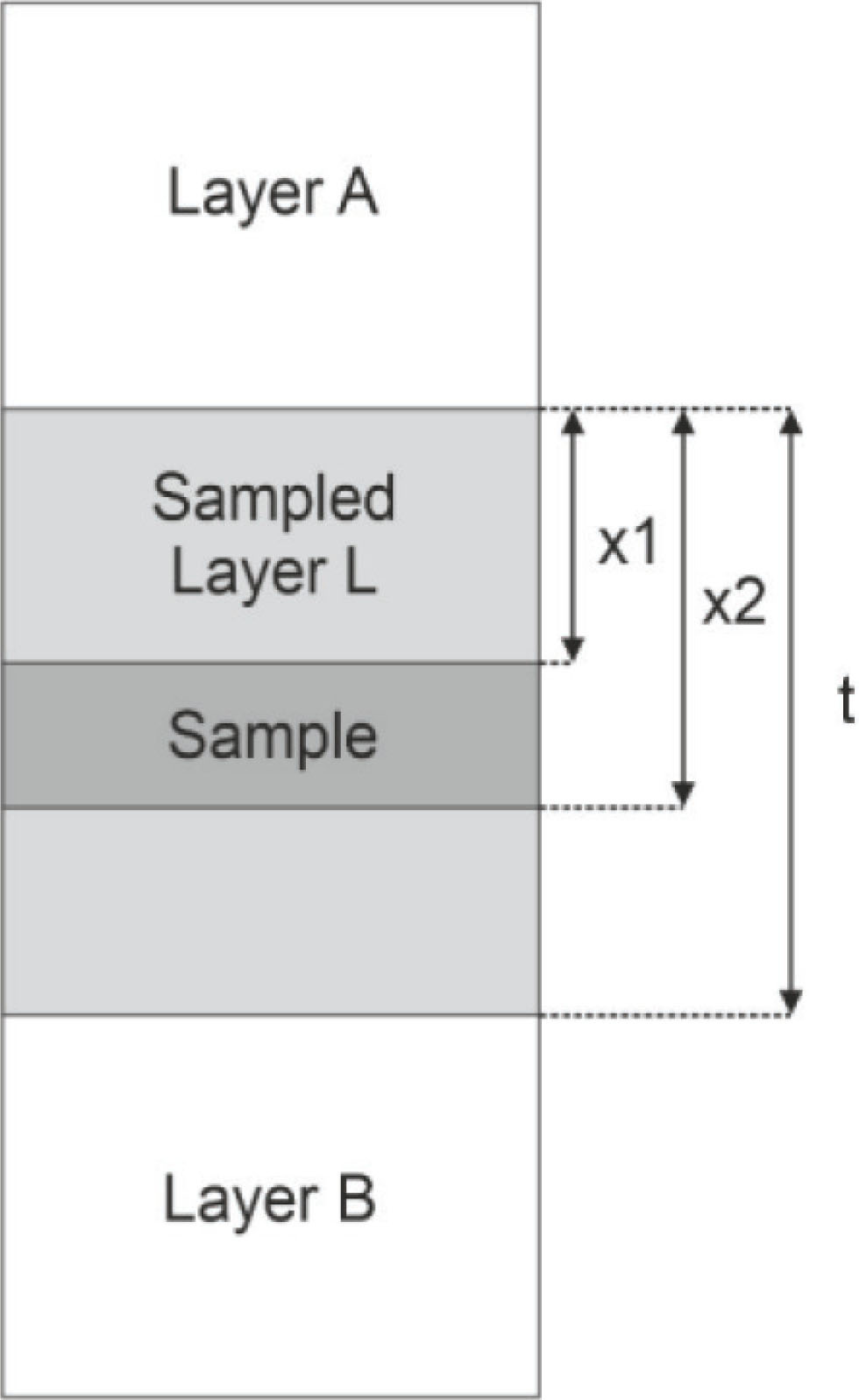
Fig 9.
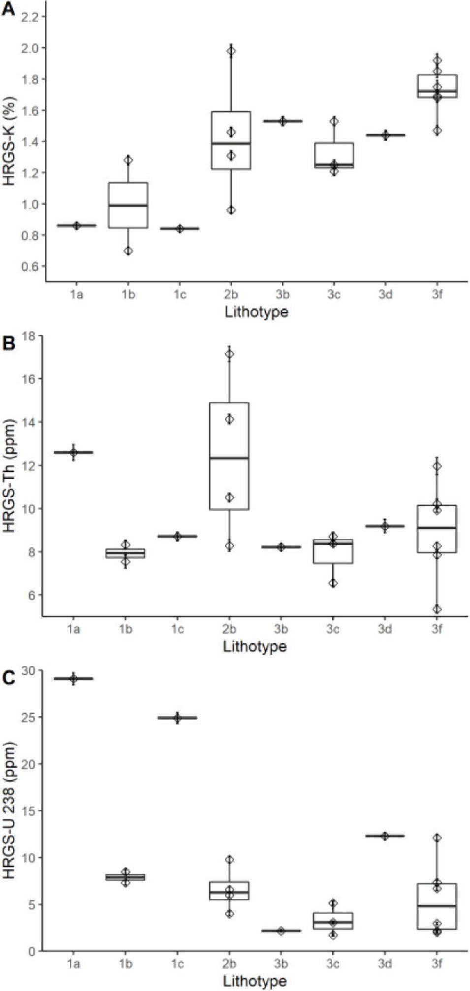
Boxplots of the radionuclide content of each LT. (A) – Potassium, (B) – thorium, (C) – uranium. Note the high variations in K and Th content for LT 2b (silty, organic-rich clays). HRGS, high-resolution gamma spectrometry; LT, lithotype.
The layer models for the samples from the two studied cores are illustrated in Fig. 7. For three samples from core NW2018/2, the layer model is simplified to a two-layer model, while the remaining nine samples are described by a three-layer model. Only one sample from core NW2018/3 is described using a two-layer model, while the other six samples are described by three-layer models. Between 3 m and 4 m depth, there are several very thin sediment layers, and therefore, the layer model for the samples NW18/3-21 and NW18/3-10 likely simplifies the true inhomogeneous radiation field. For example, for samples taken within the finely interbedded peat-clay section at 5–6 m depth, the radiation fields would best be described by five-layer models. However, the used software can only accommodate three-layer models, in which layers A and B have an infinite extension (effectively 30 cm). However, with increasing distance from the sample, the influence of the more distant radiation sources diminishes, and thus, a simplification of the geological setting to a three-layer model appears acceptable.
For core NW2018/2, the layer model correction for the top three samples (NW18/2-09 to NW18/2-11) is not more than 200 years (max. effect on age 0.3%), and it is more relevant for some of the samples from the middle and lower parts of the core (Fig. 10). For example, the age of sample NW18/2-22 increases from 118.9 ± 9.2 ka to 122.5 ± 9.7 ka (3.6 ka, 3.0%), NW18/2-23 increases from 37.5 ± 3.7 ka to 39.9 ± 4.2 ka (2.4 ka, 6.4%) and NW18/2-25 decreases from 164.1 ± 10.6 ka to 155.1 ± 9.5 ka (9 ka, 5.5%). The most prominent effect is observed for sample NW18-2-24, where the ages decrease from 124.6 ± 6.6 ka to 114.5 ± 10.1 ka (10.1 ka, 8.1%). For core NW2018/3, a larger effect is observed for sample NW18/3-21, where the age increased from 79.7 ± 5.8 ka to 86.0 ± 6.7 ka (6.3 ka, 7.9%), whereas most samples show no relevant change after layer correction (Fig. 10).
Fig 10.
Illustrating the impact of layer correction on the IRSL ages of core NW18/2 (A,B) and NW18/3 (C,D), both given as absolute values and a ratio in comparison to the age calculated without layer correction (using the estimated water content, as discussed in Section 4.2). IRSL, infrared stimulated luminescence.
. Radioactive Disequilibrium
Radioactive disequilibria were detected solely in the U-238 decay series since the low half-lives of all Th-232 successors results in a recovery of any disturbed equilibrium within some decades. Samples with indication of significant disequilibrium show a surplus of U-238 over Ra-226. Additional analyses of Th-230 were used to decide whether a model for radium loss or for uranium uptake must be chosen. The long-term measurements at VKTA Rossendorf show a clear trend of equilibrium between Th-230 and Ra-226, indicating an enrichment of U-238.
Radioactive disequilibria indicate the occurrence of an open system, either at deposition and/or during certain periods after deposition. The mass exchange of open systems is generally linked to migration processes in the aqueous phase. Both uranium and radium are soluble under oxidising conditions, whereas thorium is virtually insoluble (cf. Ivanovich and Harmon, 1992). Because of their half-lives, U-238/Th-230 disequilibria exist for some 100 ka, whereas Th-230/Ra-226 imbalances disappear after about 10 ka.
Only uranium uptake in open systems thus explains the observed disequilibria; any Ra loss in the past cannot be excluded but is at present no longer detectable. In the applied models, we assume the presence of two phases: a mineral detritus showing a radioactive equilibrium and an additional phase (e.g. organics) with the ability of uranium accumulation. The detrital uranium content was derived from the thorium content of the sample, using the ratios found in the equilibrated material. Furthermore, it was assumed that open system behaviour was in the past limited to periods without permafrost or long-lasting seasonal ground frost. While permafrost was most likely present in central Europe during the Last Glaciation Maximum (LGM) (e.g. Murton, 2021), data presented by Andrieux et al. (2018) imply that phases with frozen ground may have persisted for much longer periods of the Late Pleistocene. Based on the reconstruction of environmental conditions (cf. Preusser, 2004; Heiri et al., 2014), we assume that open system behaviour was only possible 0–15 ka, 46–60 ka and between 70 ka and 130 ka.
With these boundary conditions, two scenarios explaining the current activity ratios were investigated:
Scenario 1: At the time of deposition (t = 0), a certain amount of detrital U-238 was present in the sample that was in equilibrium with the rest of the decay chain. In addition, uranium (U-238, U-234) was already absorbed at this time, representing a very early uptake situation. An open system with gain or loss of uranium existed only during the youngest period (15–0 ka) and resulted in the present concentration of radionuclides. A higher initial concentration of uranium would require open system behaviour during additional periods and possibly an exchange of radium. Hence, this model described the highest possible uranium content at the time of deposition.
Scenario 2: At the time of deposition, the U-238 decay chain is in radioactive equilibrium at the level equal to the detrital value. Exchange of uranium was possible during three periods (P5 > 70 ka, P3 = 60–45 ka, P1 = 15–0 ka), whereas the system remained closed during times of permafrost. Due to the presence of peat and based on the results by Dehnert et al. (2012), it is assumed that it is very unlikely that the investigated sediment pre-dates MIS 5 (= 130 ka).
The effect of dose rate correction using the two different scenarios is illustrated in Fig. 11. For core NW18/3, effects are on the order of few% with the exception of sample NW18/3-22 (8 ka, 9.1%). For core NW 18/2, which contains several more organic-rich layers, the presence and effects of disequilibria are much more pronounced. Here, for 7 out of 11 samples, the effect of disequilibrium on the age estimate is 5%. Interestingly, both an up-take (NW18/2-10, NW18/2-09, NW18/2-23, NW18/2-07, NW18-2-24, NW18/2-06, NW18/2-25, NW18/3-11, NW18/3-22) and a loss (NW18/2-11, NW18/3-09?) of uranium are observed. However, for some samples, the results of gamma spectrometry, also in comparison with the NAA data, are ambiguous (NW18/2-21, NW18/2-08, NW18/2-22) or point towards no significant disequilibrium (remaining samples). The most important effect is observed for sample NW18/2-8, with 18% (scenario 1) and 24% (scenario 2) higher age estimates.
Fig 11.
Illustrating the impact of different scenarios of correction for radioactive disequilibrium on the IRSL ages of core NW18/2 (A,B) and NW18/3 (C,D). The central column represents a simplified stratigraphy of the sediment sequence for comparison; details are given in Fig. 6. IRSL, infrared stimulated luminescence.
. Discussion
The assignment of OSL and IRSL ages to the sediment sequences after ultimate dose rate correction is displayed in Fig. 11, a summary of the different dose rates calculated is found in Table 5, whereas mean De values and resulting ages are given in Table 6. The age-depth plots show a fundamentally different picture for the two different cores investigated, which will be discussed separately.
Table 5.
Calculated dose rate data with sample code and composite depth, and estimated long-term water content.
[i] Dose rates are given for both quartz (Q) and polymineral fine-grains (F) for three different scenarios: (1) using ‘standard’ scenario with estimated water content, (2) using estimated water content and layer correction and (3) estimated water content, layer correction and considering radioactive disequilibrium with the uncertainty related to the two different scenarios (given are the lower and upper dose rate estimates, which share the same uncertainty).
Table 6.
Mean De values (CAM) and resulting ages with sample code, composite depth and number of replicate measurement (quartz/feldspar) for OSL and IRSL.
[ii] Ages were calculated using three different scenarios: (1) using ‘standard’ scenario with estimated water content, (2) using estimated water content and layer correction and (3) estimated water content, layer correction and considering radioactive disequilibrium, with the uncertainty related to the two different scenarios (given are the lower and upper age estimates, which share the same uncertainty).
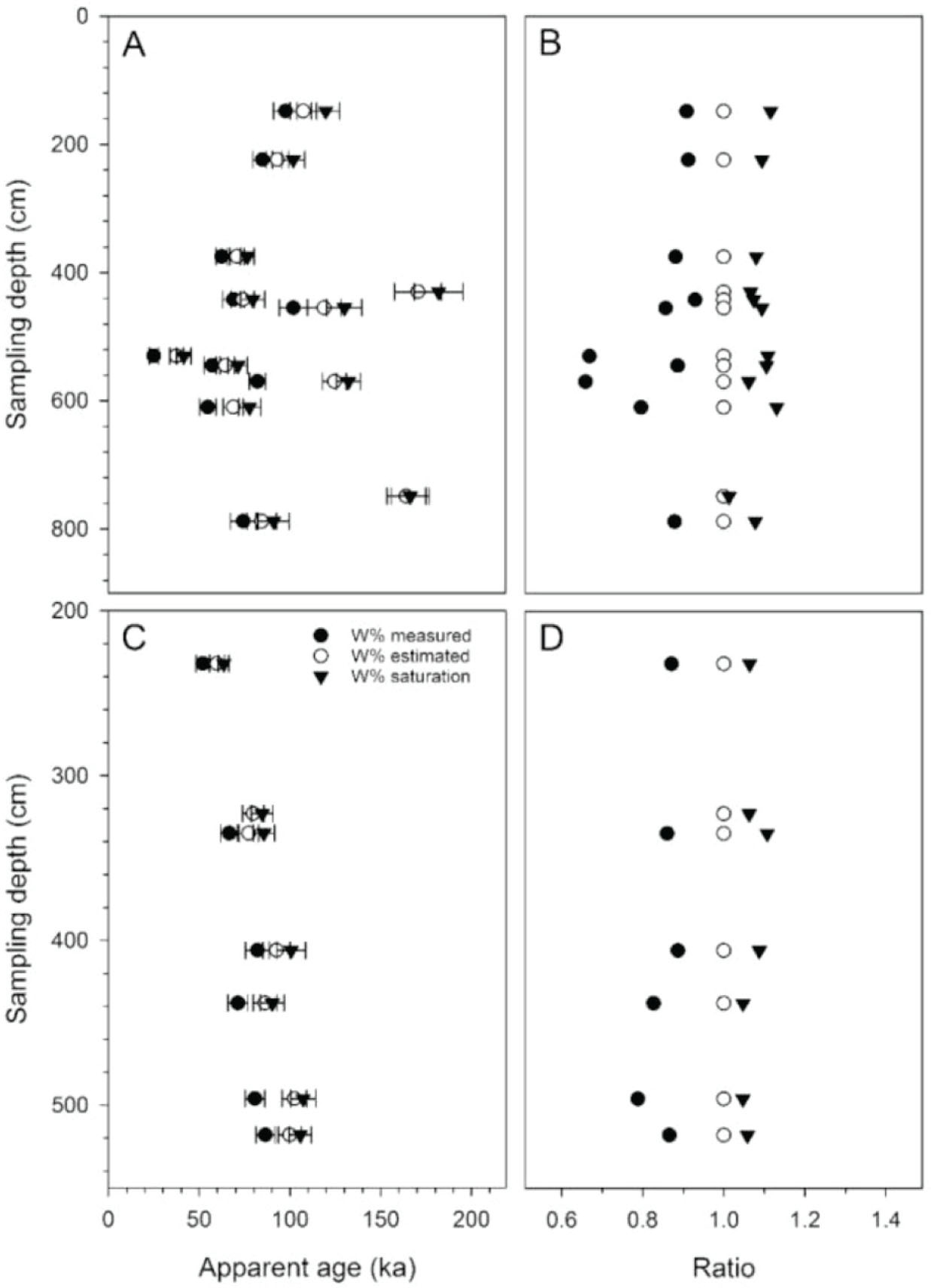
For core NW18/3, the quartz OSL ages show a steady increase with depth from 70.5 ± 3.5 ka to 101 ± 4 ka. For polymineral IRSL, the increase in age with depth is a little less uniform, but overall, there is a very good agreement between the two approaches; the ratio of IRSL/OSL ages is 1.01 ± 0.12. This is despite the lack of fading correction for the present data set, but not applying such a correction is in agreement with previous reports from Niederweningen (Anselmetti et al., 2010; Dehnert et al., 2012). While there is a tendency of higher De values determined of polymineral fine-grains (Fig. 3D), this is explained by the higher (ca. 10%) dose rate due to larger a-values (polymineral: 0.07 ± 0.02; quartz: 0.04 ± 0.01). Dehnert et al. (2012) report significantly higher IRSL than OSL ages in the bottom part of the lacustrine sequence, which has been deposited in a proglacial setting (this part of the sequence is not investigated here). These authors argue this is likely explained by incomplete bleaching of the IRSL signal in turbid waters. Following this argumentation, we conclude that the overall consistency of IRSL and OSL ages indicates the absence of partial bleaching in the present samples. It should be noted that for the part of sequence investigated here, Dehnert et al. (2012) also did not observe any indication of partial bleaching.
The different dose rate corrections carried out within the frame of this study have, for core NW18/3, only a minor to moderate effect, not exceeding 10% of the final age estimate. According to the dating results, core NW18/3 covers the period ca. 100–70 ka; hence, most of the Early Würmian including its two well-developed interstadials (cf. Preusser, 2004). These apparently reflect equivalents of the Brørup and Odderade of northern Central Europe. Neglecting the dose rate corrections would not have led to a different interpretation, and overall the chronological assignment appears reliable.
For core NW18/2, the situation is very different. The age data set is internally highly contradictory, both with regard to stratigraphic inconsistencies and some moderate conflicts between OSL and IRSL ages, the IRSL/OSL age ratio is 1.07 ± 0.15. Interestingly, age discrepancies within the sequence become often even more pronounced after applying dose rate corrections, that is, opposite of what was expected and what represented the initial motivation for this entire study. This requires a detailed discussion of individual data before conclusions considering the applied procedures and implications regarding the age assignment can be drawn.
For the basal part of the core, two samples have been investigated, one at a depth of 788 cm (NW18/2-05) at the top of rather homogenous silty (lacustrine) deposits, and one at 749 cm depth (NW18/2-25) within a sequence of silty and peaty layers. The first sample is neither significantly affected by layer correction nor is there any indication for radioactive disequilibrium. Hence, the IRSL age of 84.4 ± 5.5 ka appears at a first glance reliable. For sample NW18/2-25, there is quite some effect from layer correction and radioactive disequilibrium, which leads to a decrease in the final corrected OSL and IRSL ages of just below 10%, compared to the uncorrected age estimates. The ages after correction of 134 ± 7 ka (OSL) and 151 ± 11 ka (IRSL) just overlap within uncertainties. The tendency towards slight discrepancy of ages could be explained by the effect of partial resetting of the IRSL signal, as suggested by Dehnert et al. (2012). Overall, there remains uncertainty with regard to the age of the basal part of core NW18/2. While the apparently unproblematic sample NW18/2-05 points towards an onset of deposition during MIS 5c (ca. 85 ka), with regard to dose rate, the OSL age of the more challenging, sample NW18/2-25 rather points towards a start of deposition during MIS 5e (ca. 130 ka). The latter interpretation would concur with an apparently obvious model, according to which the basin of Niederweningen would have been formed by a glaciation during MIS 6, followed by filling with sediment and turning it into a peatland (cf. Dehnert et al., 2012). However, both Anselmetti et al. (2010) and Dehnert et al. (2012) also observe evidence for potential lacustrine deposition after the Last Interglacial, and the available data do not allow closing this controversy.
The lower central part of the sediment sequence, between 610 cm and 530 cm depth, is covered by four samples, for which only IRSL ages could be determined. All samples are apparently only to a minor, or at worst to a moderate, degree affected by layer heterogeneity and/or radioactive disequilibrium. Two of these samples have consistent IRSL ages of 70.8 ± 5.6 ka (NW18/2-06) and 69.4 ± 5.2 ka (NW18/2-07), whereas the sample located between these two has a significantly higher IRSL age of 102 ± 9 ka (NW18/2-24). While the first two ages point towards a correlation of this part of the sequence with late MIS 5a (85–71 ka), the older sample would attribute this part to MIS 5c (102–91 ka). Entirely outside of the rest of all other samples is the IRSL age of 32.4 ± 3.4 ka for sample NW18/2-23. This sample shows both the lowest De value of the entire data set (148.9 ± 5.5 Gy) and the highest dose rate (3.73 ± 0.39 Gy ka−1). Striking for this sample is the high U-238 concentration (29.03 ± 0.64 ppm) and the clear evidence of radioactive disequilibrium (daughter isotopes at 15.24 ± 0.27 ppm). A mechanism to explain the low age could be a very late but extremely high U-238 uptake, but calculating any scenarios for this would be arbitrary in the absence of supporting information. Nevertheless, for other samples with evidence for disequilibrium, a late U-238 uptake would also have a significant effect on age calculation that is not covered by the presented data, which is based on the scenarios most reasonably to be expected.
The upper central part of the sequence, between 500 cm and 390 cm depth, is characterised by organic-rich and very fine-grained (fine silt and clay) clastic deposits (palustrine). A clastic layer sampled within the peaty layer at 455 cm (NW18/2-22) and 442 cm (NW18/2-08) returned ages of 115 ± 9 ka (OSL), 139 ± 10 ka (IRSL) and 96.3 ± 7.6 ka (IRSL). These samples are, only to a minor extent, affected by layer inhomogeneity and moderately by radioactive disequilibrium and indicate an early MIS 5, possibly Last Interglacial (MIS 5e) age. However, the sample taken slightly higher, at 430 cm (NW18/2-21), has a corrected age of 197 ± 13 ka. It should be noted this is mainly due to the enormously high water content of 180 ± 10% assumed for this organic-rich sample (51% organic matter). Present moisture was not measured for this sample as it had dried out almost entirely during storage. Using a much lower but likely still possibly reasonable water content for this particular setting would dramatically lower the age but not younger than early MIS 5.
The upper part of the sequence (from 390 cm to 120 cm depth) is composed of quite homogenous clastic fine-grained deposits with organic matter contents not exceeding 5%. While there is some evidence for radioactive disequilibrium, dose rate correction has only a minor effect on the ages. While the ages show some scatter, the mean (CAM) of all six OSL and IRSL ages of 90 ± 6 ka for this upper part of the sequence corresponds to MIS 5b (91–85 ka), the cool period separating the two Early Würmian interstadials.
. Conclusions
This study has focussed on dose rate determination in what Brennan et al. (1997) called ‘lumpy environments’. First, the comparison with certified standard material and crosscheck with NAA analyses implies a reliable performance of the applied HR-GS for the determination of dose rate-relevant elements. Second, it is shown that the present-day moisture content and water uptake capability may significantly deviate from each other for fine-grained, and in particular organic-rich deposits, raising the question which value to prefer. Likely, none of the two values will represent the real average value over the entire burial time considering changes in past environmental conditions. Approximating the average value is apparently the only solution but may represent a potential source of error, in particular for problematic samples presented here (fine-grained and rich in organic matter). Third, layer inhomogeneity has for most samples not more than a moderate effect in this case study, but this might be different in a setting where the concentration of dose rate-relevant elements shows a more pronounced interlayer variability. Forth, the major challenge in correcting for radioactive disequilibrium in the uranium decay chain is related to long-term environmental changes, that is, the question when uranium absorption or loss may have happened and at what rate. A reconstruction appears only possible in part as some sedimentary layers seem to have experienced very specific conditions in the past compared to close-by units, that is, the rate of uranium uptake might have varied on temporal and spatial scales within the sequence. This in combination with other factors likely explains the inconsistent data set observed for one of the cores investigated here. Based on the reported luminescence data, the sequence of interest investigated in core NW18/3 is attributed quite securely to the period 100–70 ka, that is, the middle to late parts of the Early Würmian (MIS 5c to 5a). The age assignment for core NW18/2 is more ambiguous, but deposition possibly occurred between ca. 130 ka and 90 ka, that is, during the early to middle parts of the Early Würmian (MIS 5e to MIS 5b).