
. Introduction
The Tatra Mountains are located in the northernmost part of the Western Carpathians and represent a typical alpine landscape that developed during the Pleistocene glaciations. The reconstruction of glaciation events and related deposits in the mountains and their foreland have been the focus of numerous studies since the 19th century (e.g. Zejszner, 1856). However, the most important findings on the Quaternary evolution of the Tatras emerged in the second half of the 20th century as a result of geomorphological and geological studies and mapping campaigns. Based on morphostratigraphic criteria and other relative dating methods (e.g. degree of clast weathering, correlation of stratigraphic horizons and pollen analyses) the studies described the Lower, Middle and Upper Pleistocene glacial and glaciofluvial deposits, recording a complex glacial history of the Tatra Mountains (e.g. Lukniš, 1964; Klimaszewski, 1988; Halouzka, 1989; Krzyszkowski, 2002; Bińka and Nitychoruk, 2003; Lindner et al., 2003). During the last two decades, the understanding of the evolution of the Tatras during the last glacial cycle has significantly been increased by using absolute dating methods for obtaining numerical ages, mostly by cosmogenic and radiocarbon dating (Makos et al., 2014; Kłapyta et al., 2016; Pánek et al., 2016). However, the chronology of the Middle and Late Pleistocene deposits is still ambiguous and mainly based on morphostratigraphic data.
In this study, we investigate the applicability of quartz and feldspar from the Tatra Mountains for luminescence dating to elucidate the Quaternary evolution of the southern foothills of the Tatra Mountains, as well as understanding its structural evolution by integrating other geological and geomorphological data (e.g. Pánek et al., 2020). We use luminescence dating and sedimentological analysis of deposits in the Biely Váh valley and the lower reach of Velická dolina valley at the foothill of the High Tatras to address luminescence characteristics of quartz and feldspar, signal saturation and sediment bleaching that affect the quality of luminescence ages. Moreover, the implications of the resulting ages for the depositional history of the sediments and their relationship to glaciations in the Tatra Mountains are discussed.
. Regional Setting
. The Tatra Mountains
The Tatra Mountains, extending along the Slovakian–Polish border, are the highest mountains of the Carpathian chain. They consist of the Western and Eastern Tatra Mountains, which are further subdivided into the High Tatra and Belianske Tatra Mountains (Mazúr and Luknis, 1978). The mountains form an asymmetric horst with a crystalline core in the southern part and Mesozoic rocks in the northern part. The crystalline core mainly consists of granitoids in the eastern part of the mountains and metamorphic rock in the western part. The mountains were intensively glaciated during the Pleistocene with 55 glacial systems during the Last Glacial Maximum (Zasadni and Kłapyta, 2014). Quaternary sediments are found in significant amounts in the southern foothills of the High Tatra Mountains. Their thickness is controlled by the topography of the pre-Quaternary basement and syndepositional tectonics (Halouzka in Nemčok et al., 1994). The Lower to Upper Pleistocene sediments were deposited in glacial and pro-glacial settings by glaciers in the mountain valleys and glacier-related rivers on the outwash plains of the mountain foreland. These deposits are characterised by extremely variable grain sizes and sedimentary facies, reflecting contrasting flow conditions and flow unsteadiness (e.g. Maizels, 1993).
Geomorphological and geological data are evidence of several glaciated periods during the Pleistocene in the Tatra Mountains, interpreted to represent two to three (e.g. Lukniš, 1973; Klimaszewski, 1988) or up to eight glaciations (Halouzka, 1992; Nemčok et al., 1993; Lindner et al., 2003). Lindner et al. (2003) state that throughout the Late Pleistocene (Würm c. 24.000–10.000 BP), a remarkably extensive glaciation took place in the Tatra Mountains. However, the remnants of strongly weathered till clasts beyond the Würmian terminal moraines suggests the maximum extent of glaciers occurred in a pre-Würm stage (Lukniš, 1968; Zasadni and Kłapyta, 2014). The Lower to Middle Pleistocene glacial history is mostly inferred from geological and geomorphological mapping (Lukniš, 1973; Klimaszewski, 1988; Nemcok and Nemcok, 1994). The occurrence of glaciations from that period is evidenced by glaciofluvial deposits on the foothills of the Tatra Mountains and strongly weathered till clasts in the mountain valleys. Cosmogenic dating performed on moraine boulders, glacially transformed bedrock surfaces and colluvial accumulations yielded a detailed chronology for the last glaciation at several places in the Slovakian part of the Tatra Mountains (Makos et al., 2014; Engel et al., 2015; Makos et al., 2016; Pánek et al., 2016). Data from the Velická dolina valley suggest that the glacier reached its maximum extent around 26–23.5 ka during the Würm glaciation (Makos et al., 2014). Small glacier advances took place before the end of the Last Glacial Maximum (c. 18 ka), and the glaciers disappeared before the beginning of the Holocene (ca. 16–13 ka) (Engel et al., 2015).
. The Biely Váh Valley and the Velická dolina Valley
The valley of the Biely Váh river (downstream from the Važecká dolina valley) originates from the southeastern foothill of the Kriváň štít peak (2495 m a.s.l.) and becomes the Váh river in the south (Fig. 1). The main study site at the Biely Váh river is located about 4.2 km WNW of the village Tatranska Strba (Fig. 1). The valley is surrounded by sediments of Würmian age in its upper part and moraines of inferred Middle (Riss) and Late Pleistocene age at the head of the valley (Nemčok et al., 1994).
Fig 1.
Map of the High Tatras where both study areas are indicated: hashed black lines indicate the area of the Velická dolina valley that covers all the six sample sites, and the yellow square indicates the Great Yellow Wall (Fig. S1). Likewise, the location of the Bee Pit is a yellow square.
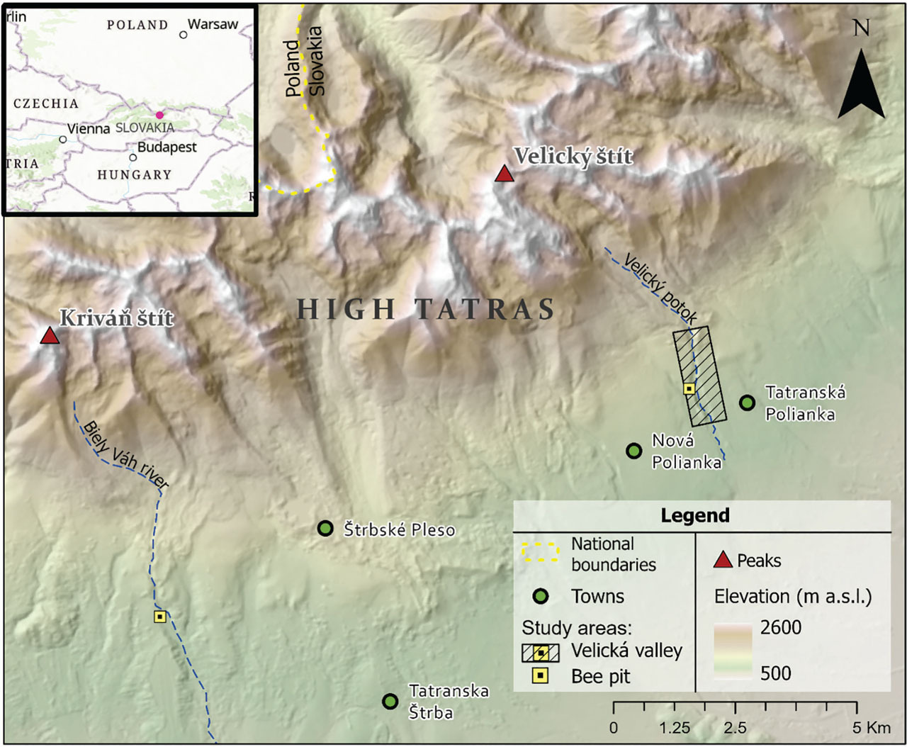
The Velická dolina valley extends from the foothill of the Velický štít peak (2319 m a.s.l.) located in the main ridge of the High Tatra Mountains. In the upper part of the valley, the Velický potok stream incises into granodiorites and borders our main stratigraphic site, the so-called Great Yellow Wall (GYW) in the lowest part of the valley (Fig. 1). The GYW consists of deposits resulting from several sedimentary processes of uncertain age and borders Late Pleistocene glaciofluvial sediments in low-lying terraces on the east (Nemčok et al., 1994). Lukniš (1974) assigned the lower part of the GYW to the Middle Pleistocene and the upper part to the Late Pleistocene. The youngest ages of moraine boulders from 1660 m a.s.l. to 1685 m a.s.l. (16.1 ± 0.7–13.5 ± 0.9 ka) could indicate the time when the last glaciers started to retreat from the Velická dolina valley (Makos et al., 2014).
. Sites and Stratigraphy
The fieldwork in the southern foothills of the High Tatra Mountains in Slovakia was carried out during August 2019. The two areas were chosen based on the available exposed outcrops, which seemed suitable for the recovery of luminescence samples and the already available data from the nearby areas (Lindner et al., 2003; Makos et al., 2014). A brief supplemental fieldwork was carried out in July 2020.
The sampling of the Biely Váh valley was concentrated on one stratigraphic site (informally named the Bee Pit after the apiculture next to the outcrop; N49.0998°, E20.0176°) that is located in a gravel pit (Fig. 1). In the Velická dolina valley, we focussed on two sites within the large sediment exposure, the GYW, in the western valley side (49.127806° 20.170897°) (Fig. 1). We also conducted additional measurements and sampling in four different sites with sediment deposits downstream of the GYW and at one site at a moraine upstream the GYW (Table 1).
Table 1.
Sample information acquired from the investigated study areas. Lithofacies codes are based on Krüger and Kjaer (1999).
| Sample No. | Site | UTM 33N easting | UTM 33N northing | Location / Sample type | Depth in m (overburden sediment) | Stratigraphic unit | Lithofacies | Fraction (μm) |
|---|---|---|---|---|---|---|---|---|
| 19082 | Bee Pit | 42829 | 5439202 | Lower section | 7.1 | B3 | SiSm(ng) | 180–250 |
| 19083 | Bee Pit | 428289 | 5439024 | Lower section | 11.4 | B1B | SSim | 180–250 |
| 19084 | Bee Pit | 428292 | 5439015 | Lower section | 13.8 | B3 | SiSm(ng) | 180–250 |
| 19085 | Bee Pit | 428289 | 5439024 | Lower section | 11.4 | B3 | SiSm(ng) | 180–250 |
| 19086 | Bee Pit | 428283 | 5439047 | Lower section | 10.8 | B3 | SiSm(ng) | 180–250 |
| 19087 | Bee Pit | 428228 | 5438971 | Upper section | 5.4 | B12 | SiSm(ng) | 180–250 |
| 19088 | Bee Pit | 428228 | 5438971 | Upper section | 5.4 | B12 | SiSm(ng) | 180–250 |
| 19089 | Bee Pit | 428228 | 5438971 | Upper section | 5.4 | B12 | Sm(ng) | 180–250 |
| 19090 | Bee Pit | 428282 | 5439016 | Lower section | 2.2 | B9 | SiSm | 180–250 |
| 19091 | Bee Pit | 428282 | 5439016 | Lower section | 2.2 | B9 | SiSm | 180–250 |
| 19092 | Bee Pit | 428286 | 5439018 | Lower section | 3.6 | B5 | Sm(ng) | 180–250 |
| 19093 | GYW, site 1 | 439489 | 5441932 | GYW South (YS) | 1.8 | YS3 | GSm | 180–250 |
| 19094 | GYW, site 1 | 439489 | 5441932 | GYW South (YS) | 1.7 | YS3 | Sm | 180–250 |
| 19095 | GYW, site 1 | 439489 | 5441932 | GYW South (YS) | 2.2 | YS3 | GSm | 180–250 |
| 19096 | GYW, site 2 | 439514 | 5442023 | GYW North (YN) | 15 | YN1 | Sm | 180–250 |
| 19097 | GYW, site 2 | 439514 | 5442023 | GYW North (YN) | 15 | YN1 | Sm | 180–250 |
| 19098 | Site 3 | 439737 | 5441549 | Flood deposit | 0.24 | - | Gm | 250–355 |
| 19099* | Site 4 | 439677 | 5441615 | East of Velická potok | 2 | - | Gm | * |
| 19100 | Site 4 | 439677 | 5441615 | East of Velická potok | 2.5 | - | Sm | 180–250 |
| 19101 | Site 5 | 439605 | 5441701 | West of Velická potok | 2.6 | - | Sh | 90–180 |
| 19102 | Site 5 | 439605 | 5441701 | West of Velická potok | 2.5 | - | Sh | 180–250 |
| 19105 | Site 6 | 439775 | 5441345 | Modern Analogue (MA) | 0 | - | Sm | 180–250 |
| 19106 | Site 6 | 439775 | 5441345 | Modern Analogue (MA) | 0.03 | - | Sm | 250–355 |
| 19103* | Site 7 | 440614 | 5436964 | Distant MA | 0 | - | Sm | * |
| 19104* | Site 7 | 440614 | 5436964 | Distant MA | 0.12 | - | Sm | 90–180 |
| 20026 | GYW, site 2 | 439514 | 5442023 | Saturated sample | 15 | YN1 | Boulder | 180–250 |
| 20028 | Site 8 | 439819 | 5442867 | Moraine | 5 | - | DmC | 180–250 |
The following descriptions and interpretations are based on the work by Bejarano Arias (2020) and van Wees (2020), where more details can be found.
. Biely Váh Valley
The lower outcrop has a width of c. 45 m and a height of 13.6 m, while the upper outcrop has a height of around 6 m. The two sections comprise 13 lithostratigraphic units and are separated vertically by around 20 m, where sediments are inaccessible due to extensive excavation-derived slope deposits as well as vegetation cover (Fig. 2). The log presents both upper and lower sections of the Bee Pit, with all the identified units and the gap in between (Fig. 3).
Fig 2.
Overview of the Bee Pit outcrop with the sampling locations in the different units. The log in Fig. 3 is from the southern side of the exposure (left in photo). The two boulders in unit 4 are marked with the red dashed line.
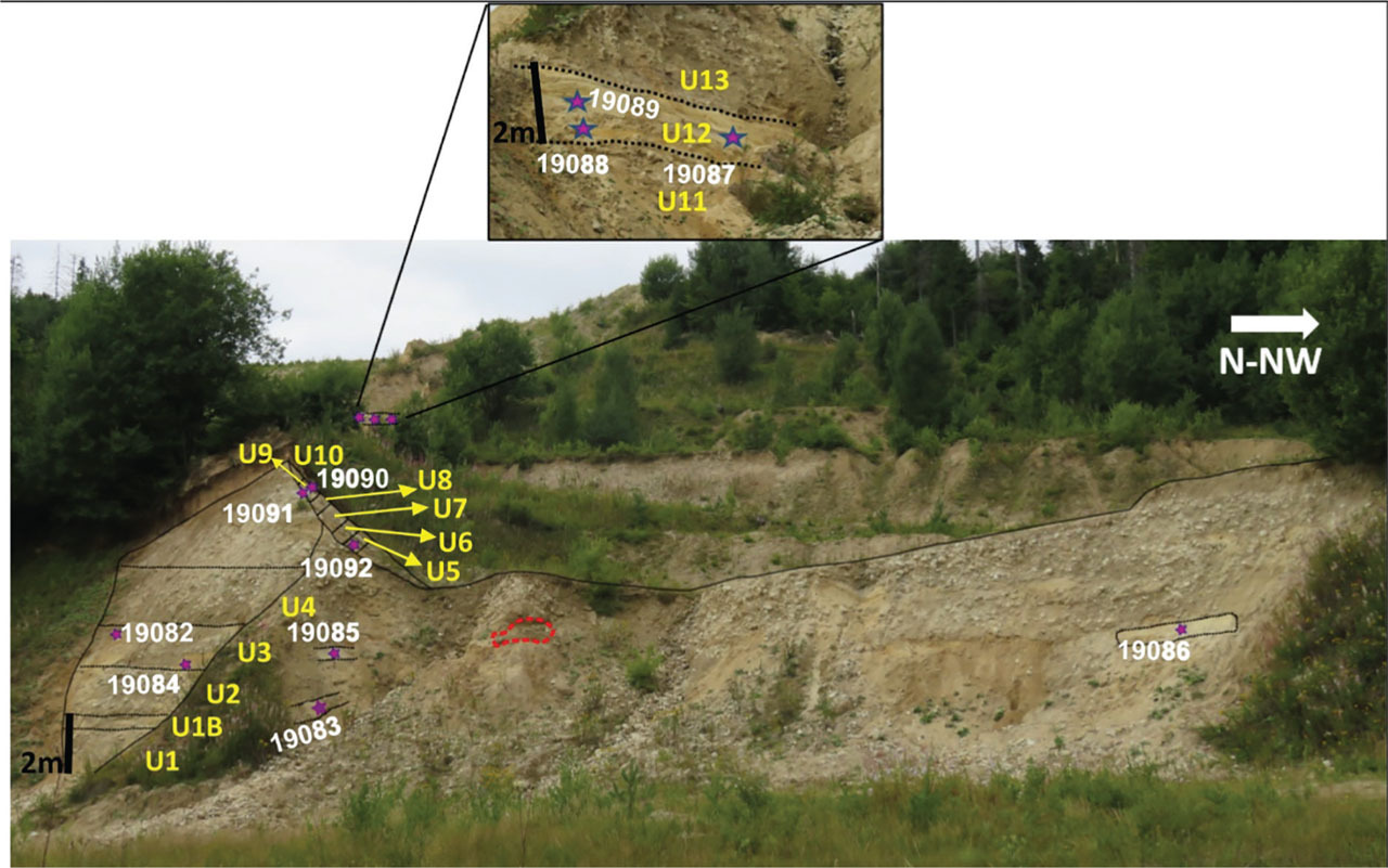
Fig 3.
Log combining the lower and upper exposures at the Bee Pit, including all units and uncorrected pIRIR225 luminescence ages from the site. The zero level in the log is approximately at 914 m a.s.l. Sample numbers and ages in bold are considered most reliable (for explanation, see text). Lithofacies codes are according to Krüger and Kjaer (1999).
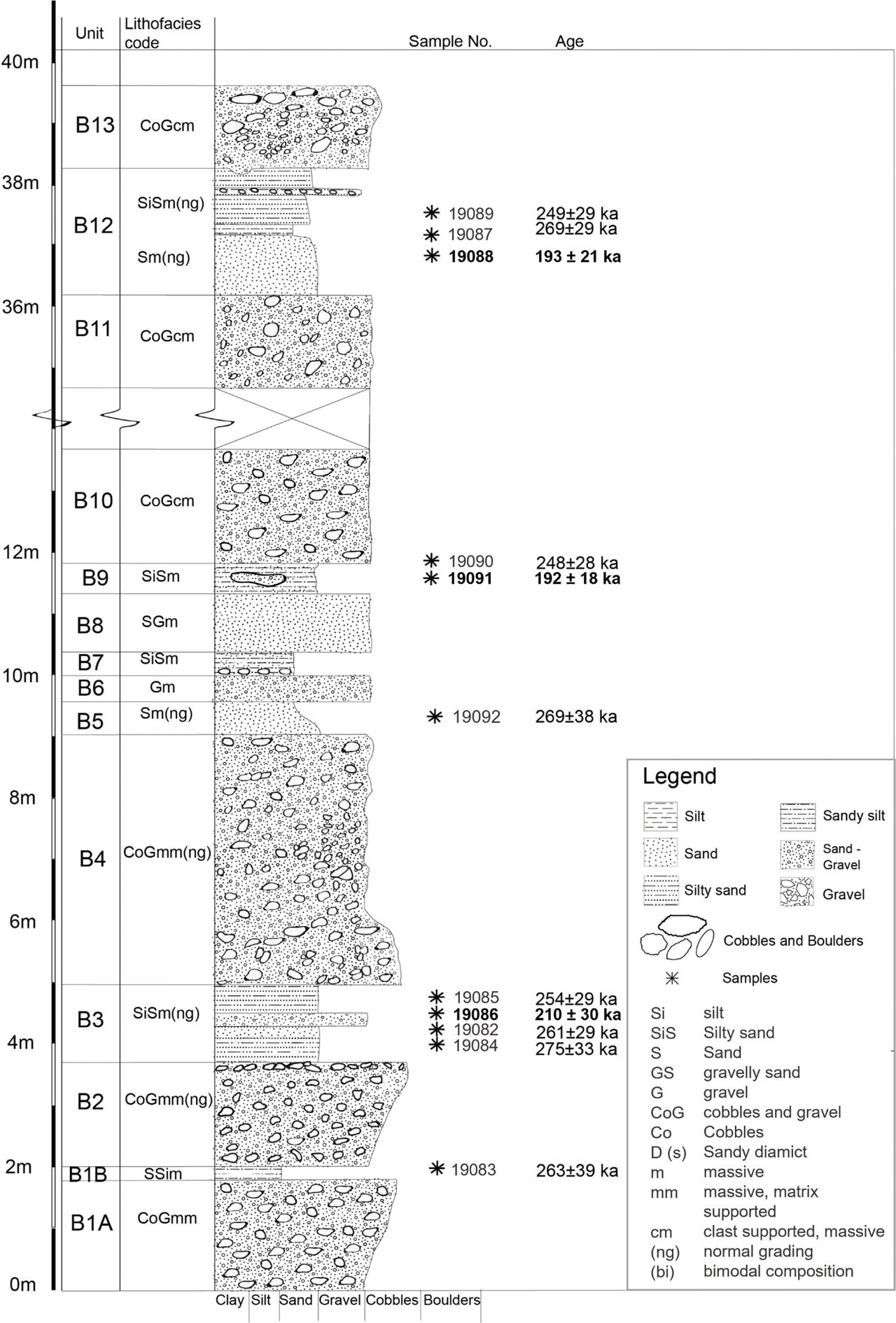
The lower section of the Bee Pit was divided into ten units, where the units B1A, B2, B4, B6, B8 and B10 are mainly composed of massive, matrix-supported cobbles and pebbles (CoGmm), while units B1B, B3, B5, B7 and B9 are composed of massive silty sand (SiSm) and sandy silt (SSim) (Figs. 2 and 3). The fine-grained units have a thickness that varies between 20 cm and 30 cm, except unit 3, which is 150 cm thick. The coarser units are c. 160–180 cm thick, except unit 4B, which has a thickness of 4 m. The coarser units present granite clasts with a high degree of weathering. Two thoroughly weathered boulders (180–230 cm in diameter) were found in unit 4 (Fig. 3). The boundaries between all units are sharp, and no faults or deformation structures were found. In the N-NW part of unit 3B, there is planar stratification in a small area, followed by incipient crossbedding.
The upper section of the Bee Pit has three units, where units B11 and B13 are composed mainly of massive, matrix-supported cobbles and gravels (CoGmm). Unit B12 is dominated by massive, normally graded sand (Sm(ng)), with minor components of SiSm towards the top (Fig. 3). The measured thickness of units B11, B12 and B13 was in total 1.6–2 m. The grain size in the coarse units ranges from pebbles to cobbles, and the clast are composed of granite, with a high degree of weathering. The boundaries between the three units are mainly sharp and partly uneven. Towards the centre of unit B12, there is a silt lens, which has an apparent planar stratification and is surrounded by granite clasts.
Interpretation: The coarse- and fine-grained sediments at both sections (units B1A, B2, B4, B6, B8, B10, B11, B13 and B1B, B3, B5, B7, B9 and B12, respectively) have common characteristics implying their similar origin. The gravel material and boulders content in these units imply that they are deposited with a high energy component. Likewise, they present the thickest layers, which also suggests an abundance of material at the time of deposition. Therefore, the coarse units are interpreted to be deposited by hyperconcentrated flows (Mulder and Alexander, 2001; Benvenuti and Martini, 2002; Benn and Evans, 2010). In the units composed of finer sediments, the grain size change indicates a fluctuation in the flow competence.
The sand layers are dominantly massive, indicating that the depositional process could have occurred rapidly. The presence of localised structures like silt lenses and normal grading indicated that their deposition had a fluvial or current component. This change was indicating the transition from hyperconcentrated to normal flow, which can occur during falling discharges, as a result of formerly suspended sediments (Maizels, 1989). Though information on the sediments from between the lower and the upper sections is missing, based on the setting and appearance of the site, we find it most likely that the upper units (B11–B13) are younger and stratigraphically overlie the lower units (B1–B10). However, based on field observations, we cannot exclude the possibility that the lower units form a (younger) terrace cut into the upper sediments.
. Velická dolina Valley
Sites 1–2 are located at the GYW, where sediments are exposed due to a mass movement (Fig. 4A). The wall is approximately 125 m wide with a height of 60 m, measured from the riverbed. The GYW exposes sediments that are part of a larger ridge running parallel to the Velický potok stream.
Fig 4.
Overview of the luminescence sampling locations in the Velická dolina valley with location of luminescence samples (yellow stars). (A) Photo of Site 2 taken from Site 1 at the Great Yellow Wall. (B) Dry riverbed north of Site 3. (C) Site 4, east from the modern river. (D) Site 5, west from the modern river. (E) Site 6, the modern riverbed can be seen in the background. (F) Overview of Site 8, showing the natural outcrop from which the moraine sample was taken.
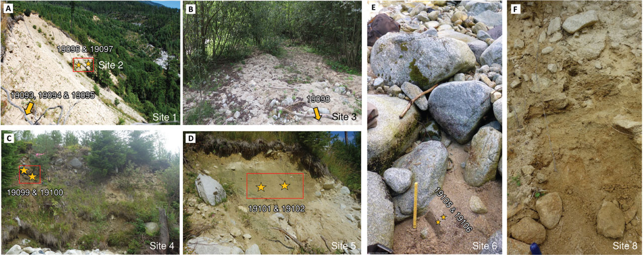
At Site 1, on the south peripheral of the GYW, four distinct lithological units were identified (Fig. 5). The two lowest units (YS1 and YS2) are massive diamicts containing sub-angular to sub-rounded clasts. Unit YS3 shows a massive, matrix-supported gravelly sand with red channelised lenses of clay and several fine sand lenses. Unit YS4 consists of clast supported boulders (size 27–78 cm), with the matrix composed of loose coarse-grained, poorly sorted sand. Luminescence samples 19093, 19094 and 19095 were all taken in unit YS3 (Fig. 5). The other units were impenetrable for sampling due to the prevalence of unweathered granitic cobbles and boulders. The poorly sorted, clast- and matrix-supported, massive diamicts of units YS1 and YS2 are interpreted as debris flow deposits (e.g. Germain and Ouellet, 2013). Unit YS2 has similar characteristics to YS1, although it is matrix supported and is still classified as a debris flow.
Fig 5.
Log from Sites 1 (left) and 2 (right), showing the units of the uppermost, southern side (YS) and the sampled northern part of the Great Yellow Wall (YN). It includes the uncorrected pIRIR225 luminescence ages, where the bold ages are the most reliable. The zero level of the log is at approximately 1110 m a.s.l., and the legend can be found in Fig. 3. Sample numbers and ages in bold are considered most reliable (for explanation, see text).
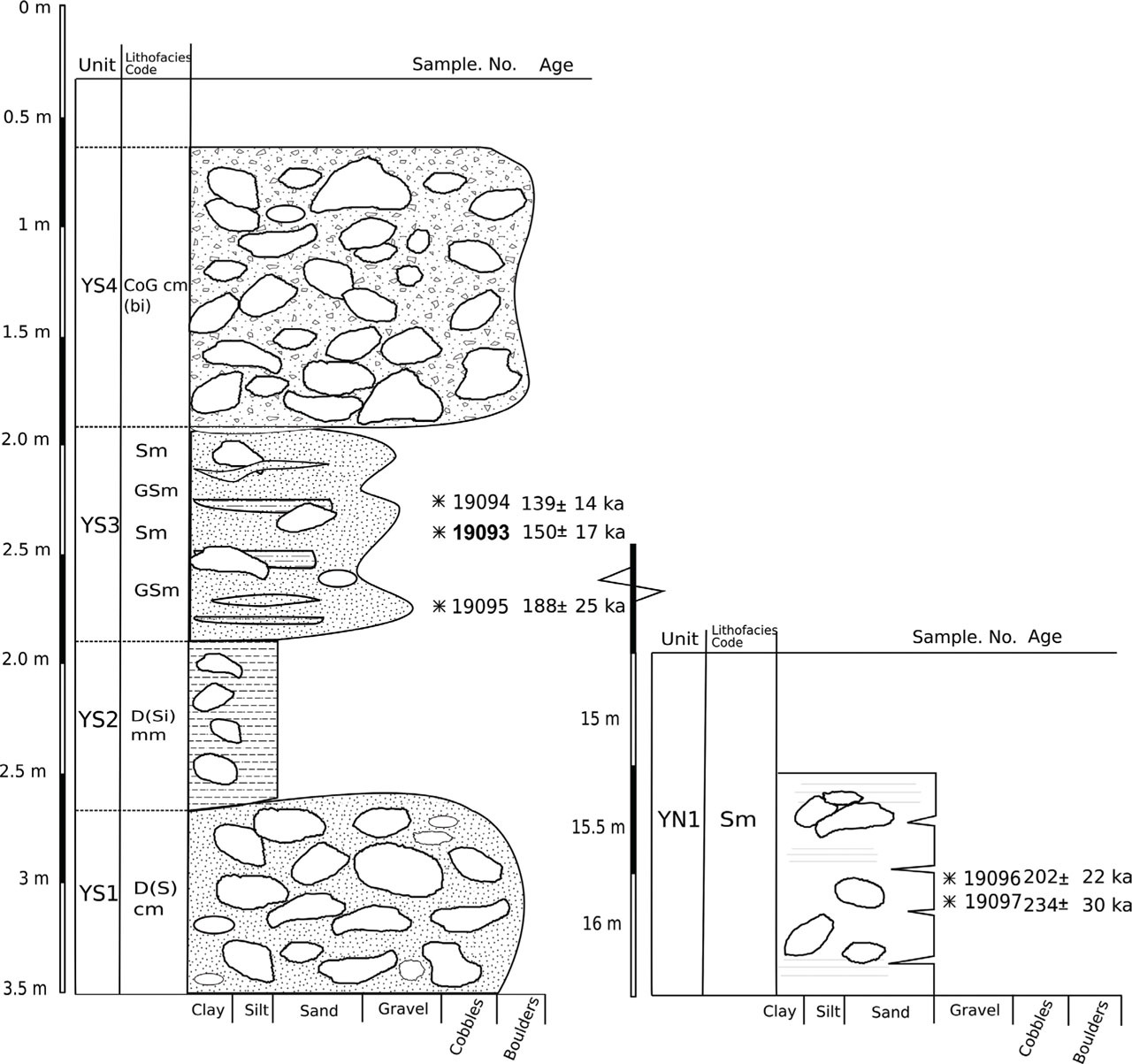
Unit YS3 contains some channelised lenses, is massive and matrix supported and therefore interpreted as a hyperconcentrated flow (Benn and Evans, 2010; Germain and Ouellet, 2013 Fig. 5). Unit YS4 resembles the boulder beds, which are found on lower elevation next to the modern river. Given the size of the boulders, the deposit is most likely deposited by a moderately powerful stream. Based on this, YS4 is interpreted as a glaciofluvial deposit.
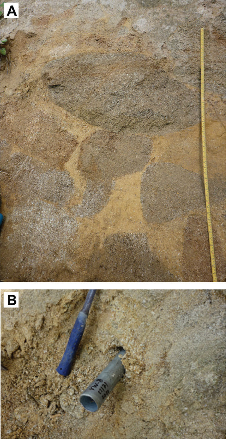
At Site 2, on the north peripheral of the GYW, around 13 meters lower than Site 1, a small section (YN1) with an area of 1.5 by 2 m was accessible for sampling. The exposed sediments consist of massive, clast-and matrix-supported boulders with a matrix composed of medium- to coarse-sized sand and granules. The boulders are strongly weathered to decomposed (Fig. 6). The general absence of pebble and cobble clasts calibre results in a bimodal appearance of the sediments. Faintly laminated medium-grained sand is visible at some areas. Samples 19096, 19097 and 20026 were collected from this site (Figs. 4A and 6A,B) containing a weak horizontal stratification. The sediment at YN1 is interpreted as a hyperconcentrated flow (Germain and Ouellet, 2013).
Fig 6.
(A) Weathered boulders with a sand matrix at Site 2, Great Yellow Wall. Sample 20026 was taken from within one of the weathered boulders and used as a sample with field-saturated luminescence signal since light exposure is not expected to have occurred at any point in time for these grains. (B) Sample 20026 taken from the weathered boulders.
Sites 3–6 are all located in the proximity of the Velický potok river. At the time of the fieldwork (August 2019), its stream was relatively turbulent, but the amount of suspended material in the water was low.
Site 3 is situated east of the river and makes up an old riverbed and side branch of the main modern stream of the Velický potok river. Sample 19098 was taken from massive medium to coarse sand at this site (Fig. 4B). Site 3 is a dry riverbed supposedly deposited during a flash flood; these floods occur regularly in the Tatra Mountains (Ballesteros-Cánovas et al., 2015). The sediments are therefore interpreted as flood deposits.
At Site 4, east of the Velický potok river, an outcrop was found on a higher level next to the river (2–2.5 m above the present-day riverbed) in what appears to be a ca. 8-m-high ridge along the valley. Two small sections of 50 by 50 cm were dug, and samples 19099 and 19100 were taken, one in each section. The material consisted of loose, massive coarse sand to fine gravel with some large boulders (>1 m) (Fig. 4C). The sediment is massive and ungraded and appears to be poorly sorted with no evidence of any deformation or sheet-like masses. Based on this, the sediment at Site 4 is interpreted as gravity-driven mass movement deposit of flowing or falling down the slope of the river valley (Benn and Evans, 2010).
Site 5 is an outcrop with an area of 3.5 by 5 m, positioned west of and 2.5 m above the present-day Velický potok riverbed. The site represents the lowest part of the ridge of which the GYW is part of in the south. The exposed sediment is laminated and consists of alternating thick laminae of medium and coarse sand. Samples 19101 and 19102 were taken with a 1.5 m horizontal distance (Fig. 4D).
Horizontally laminated medium and coarse sand suggests upper and lower flow regime plane bed conditions common in glacifluvial environment (e.g. Russell, 2007). In addition, the absence of gravel and clasts points to a relatively calm depositional environment.
Site 6 is located in the riverbed of the Velický potok, and modern analogue samples were extracted from here. At the time of sampling of samples 19105 and 19106, this part of the riverbed was dry and around 2.5 m wide; it is presumed that it deposited at a higher water level in the recent past (Fig. 4E).
Site 7 is located around 4.5 km downstream from Site 6. Samples 19103 and 19104 were sampled 2 m from the active river in medium to coarse sand and are referred to as distant modern analogues.
Site 8 is a moraine ridge in the upper part of the Velická dolina valley. Sample 8 was taken from a natural outcrop ca. 1.5 m wide and 1.4 m high located on the slope some 25 m above the left bank of Velický potok creek (Fig. 4F). The sediment consists of angular and sub-angular, polymodal pebble and cobble sized granite clasts with medium- to coarse-grained sand and granule matrix. The surface of the clasts is unweathered. The structure of the sediment is disorganised, and the clasts are predominantly clast-supported. The poor sorting and disorganised appearance of the sediment may suggest glacial deposition, which is in agreement with previous interpretations of these sediments (e.g. Lukniš, 1968; Nemcok and Nemcok, 1994).
. Luminescence Methods
. Sampling
The samples for luminescence dating were taken by horizontally hammering opaque PVC tubes into the vertically exposed sediments. In total, 27 samples were collected (Table 1). To avoid exposure to sunlight, light-proof lids and opaque bags were used to for storage. In the proximity of the tube, a soil sample ring of 100 cm3 was taken and used to measure the water content and sediment density. The surrounding material (c. 30 cm radius) from the luminescence samples was collected for dose rate determination (∼200 g per sample), including small clasts to represent any nearby clasts in the sediment. During this process, the sediment type, the coordinates (using a handheld GPS: Garmin Etrex 30), elevation, overburden sediment, and environmental surroundings were noted.
. Sample Preparation
The recovered luminescence samples were opened and prepared under subdued red light in the Lund Luminescence Laboratory at Lund University, Sweden. The sediment from the middle part of the tube was wet sieved, and the 180–250 μm fraction was extracted for most of the samples. Only for four samples from the Velická dolina valley, a finer (90–180 μm) or coarser grain size (250–355 μm) had to be used due to the sediment's grain size distribution (Table 1). The samples were first treated with 10% HCl and 10% H2O2 to remove carbonates and organic material, respectively, after which a heavy liquid solution (LST Fastfloat; 2.62 g/cm3) was used to separate quartz from feldspar grains. The extracted quartz was treated with HF (40%) for up to 60 min, followed by HCl (10%) for 40 min to remove any remaining fluorides. After rinsing, the samples were dried and then sieved again using a 180-μm sieve (or corresponding lower limit). Finally, any magnetic grains were removed with a handheld magnet.
The obtained feldspar went into a test tube with LST Fastfloat at 2.58 g/cm3 to separate K-feldspar from plagioclase. The K-feldspar fraction was treated with HF (10%) for 20–40 min depending on grain size and subsequently with HCl (10%) for 40 min. Afterwards, it underwent the same sieving procedure as quartz.
For dose rate determination, the samples were weighed after being heated to 105°C for 24 h to determine the dry weight. After that, they were ignited at 450°C for 24 h to remove organic matter. After being crushed to silt size (<20 μm), the sediment was mixed with beeswax and cast into a standard geometry (cups) for high-resolution gamma spectrometry measurements (Murray et al., 1987, 2018) at the Nordic Laboratory for Luminescence Dating at Risø, Denmark.
. Luminescence Measurements
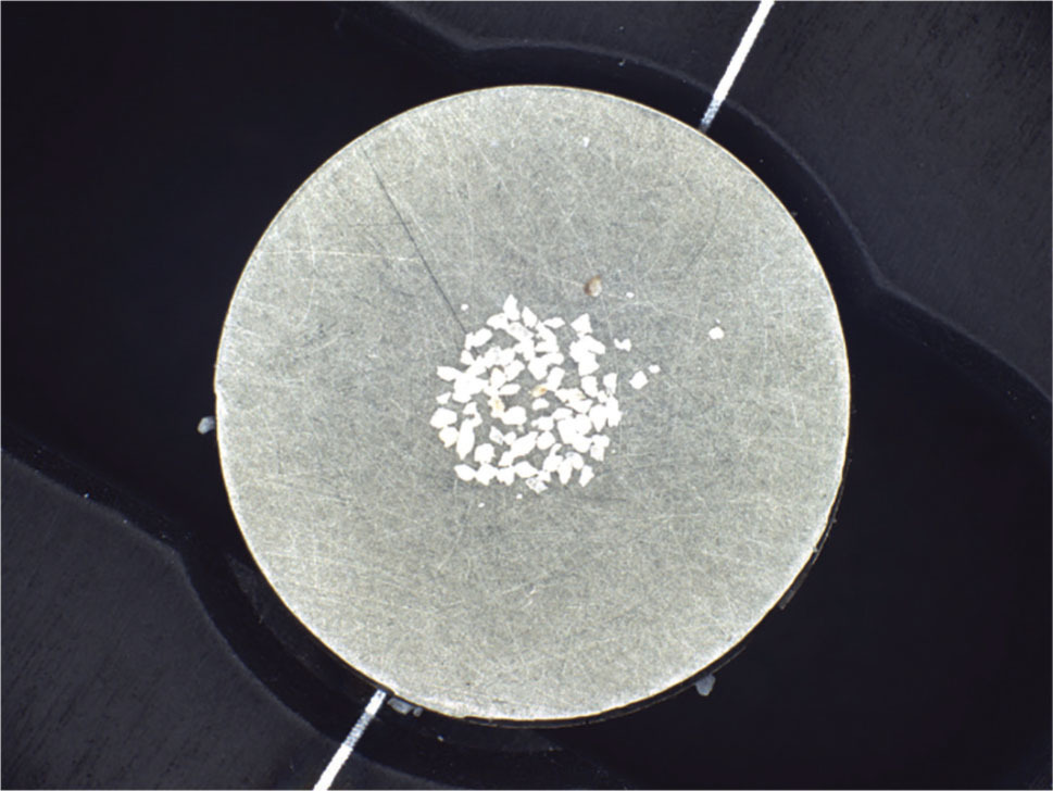
The luminescence measurements were performed using Risø ‘TL/OSL DA-20’ readers (Bøtter-Jensen et al., 2000, 2003) at the Lund Luminescence Laboratory. The readers were equipped with blue light-emitting diodes (LEDs) (470 nm, ∼80 mW/cm2), infrared (IR) LEDs (870 nm; ∼135 mW/cm2) and a 90Sr/90Y beta source (dose rates 0.16–0.20 Gy/s) calibrated for disc geometries using the Risø 180–250 μm calibration quartz (batch 123). The quartz optically stimulated luminescence (OSL) signals were collected through a 7-mm or 7.5-mm Hoya U–340 (UV) glass filter and the K-feldspar (post–IR) IRSL through a combination of Corning 7–59 and Schott BG–39 glass filters. To mount the aliquots, the stainless steel discs were sprayed with silicon spray (Fig. 7).
Fig 7.
Small (2-mm) aliquot with feldspar grains used for dose estimation of sample 19102. The average number of grains for the small aliquots is approximately 70.
The determination of equivalent dose (De) on the quartz fraction was conducted using three different approaches. Single aliquot regeneration (SAR) protocols with post-IR blue stimulation (Murray and Roberts, 1998; Roberts and Wintle, 2001) were used for most samples (19082–19092). For selected samples, pulsed OSL (Ankjærgaard et al., 2010) and differential OSL (Jain et al., 2005) were carried out to overcome problems of feldspar contamination and a weak fast signal component, respectively. All quartz samples were measured as large 8-mm (c. 1000 grains) aliquots. The feldspar contribution to the samples was assessed by calculating the ratio between the IR and the blue (B) stimulated signal (IR/B ratio) measured in nine samples from the Bee Pit and six samples from the Velická dolina valley (three aliquots per sample).
The SAR measurement sequence included preheating to a temperature of 220°C for 10 s, followed by stimulation using IR LEDs at 125°C for 100 s to monitor and deplete the IRSL signal from feldspars. Optical stimulation was carried out using blue LEDs for 40 s at 125°C. Sensitivity changes were corrected using the OSL response to a test dose (∼10–20% of the assumed natural dose) throughout the SAR protocol. All measurements included intrinsic tests (recycling and recuperation) (Murray and Wintle, 2003). Every SAR cycle was followed by a 40-second high-temperature clean-out at 280°C.
Preheat plateau (PHP) tests and dose recoveries at different temperature combinations, ranging from 180°C to 260°C for the first half of the cycle (preheat) and 160°C to 220°C for the second half (cutheat) following the SAR protocol (Murray and Wintle, 2000, 2003), were carried out on samples 19082, 19084, 19086 and 19089 to determine the most suitable preheat temperature to use for the rest of the quartz samples. Most tests were carried out on sample 19082 because it provided enough material and it belongs to unit 3 of the Bee Pit, from which several of the other samples were also taken. Dose recovery tests were conducted on aliquots that were exposed to natural light in a window (at the Department of Geology in Lund, Sweden) for 3–5 days in January and then given a known dose in the laboratory. Dose recovery was performed both for the SAR protocol and differential OSL with a given dose of 133 Gy and a test dose of 16–25 Gy. Different integration intervals for peak and background were tested, representing both early and late background subtraction. The dose–response curves for quartz samples were constructed by using exponential curve fitting function in Analyst v4.57.
Differential OSL (Jain et al., 2005) was tested on three samples (19082, 19084 and 19089) using a sequence that repeats the whole cycle with three increasing doses (64, 128 and 192 Gy), followed by a zero dose. For pulsed OSL measurements, a gated pulsed stimulation using on and off time settings each of 50 μs (i.e. a pulse period of 100 μs) was used (samples 19082 and 19102). For the standard SAR and pulsed measurements, aliquots were accepted if the recycling ratio was within 10% of unity and the test dose error was 10%. The recuperation signal was considered acceptable at a value of <5% of the natural signal.
To get a better understanding of the luminescence behaviour of quartz from the Tatra Mountains, we investigated the thermal stability of the quartz OSL signal by performing a pulse–anneal experiment on one representative sample (three aliquots per sample) from each investigated site: 19082 from the Bee Pit, 19095 from the GYW and 19104 from Site 7, which also represents a modern analogue. Electrons were evicted from the OSL traps by heating the samples to 500°C, after which a laboratory dose of 80 Gy was given. The aliquots were then preheated for 10 s between 220°C and 440°C at 20°C increments, followed by OSL measurement at 125°C for 40 s. A final 500°C heat treatment was performed after each run to remove any remaining signals. The correction for sensitivity changes during the pulse–annealing experiments was made using OSL response to a test dose of 8 Gy. The luminescence remaining after heating to each temperature was normalised to the initial value. For comparison, the same experiments were conducted on two aliquots of the Risø calibration quartz (batch 123), which is known for a strong fast component (Hansen et al., 2015). For the calculation of the OSL intensity, the initial 0.1 s (1.0–1.1 s) of the decay curve minus an early background (1.2–1.3 s) was used.
We also analysed the individual components of the OSL signal using linear modulated (LM) OSL measurements on the same samples as for the pulse–anneal experiment. For comparison, we also performed an LM measurement on the Risø calibration quartz (Batch 123) and calculated the fast ratio according to Durcan and Duller (2011) for all quartz samples, except sample 19103.
For the LM-OSL measurements, the quartz grains were first irradiated with a laboratory beta dose of 50 Gy, after which a 200°C preheat for 10 s was applied. The LM-OSL signals were subsequently measured for 1000 s at 125°C while linearly increasing the power of the blue LEDs from 0 mW/cm2 to 65 mW/cm2. For the background determination, one additional blank aliquot was measured in the same manner as the quartz grains. The deconvolution of the LM–OSL curves was performed using the fit_LMCurve function of the R Luminescence package (Kreutzer, 2022 in, Kreutzer et al., 2022). The data were fitted according to the equation of Bulur (1996):
where L(t) represents the luminescence intensity as a function of time t, Ai is the amplitude, bi is the detrapping probability (which is proportional to the photoionisation cross–section σi and the maximum light intensity I0; bi = σi. I0) and P is the total stimulation time. The contribution of the fast component to the initial signal was determined using Analyst v4.57 (Duller, 2018).All feldspar measurements were performed using small 2-mm (50–100 grains) aliquots (Fig. 7). Dose determination was performed following the SAR protocol of Buylaert et al. (2009), with post-IR IR225 stimulation (pIRIR225). After a preheat of 250°C for 60 s, the aliquots were stimulated twice with IR diodes for 100 s. The temperature during the first stimulation was kept at 50°C (IR signal). The second IR stimulation temperature was held at 225°C. The response to the test dose (16–29 Gy) was measured in the same manner. To reduce recuperation, an IR illumination (clean-out) at 290°C for 40 s was administered at the end of each SAR cycle. Doses were calculated for both IR50 and pIRIR225, and representative dose–response curves for the IR50 and pIRIR225 signals are presented in Figs. 8A,B, respectively. Dose recovery tests were carried out on samples that have previously been exposed to daylight in a window for 7 days (given dose 250 Gy, test dose 16 Gy). Aliquots were accepted if the recycling ratio was within 10% of unity, test dose error was <10% and the maximum recuperation was <5% of the natural signal. Anomalous fading was measured using the same aliquots as for De determination on all samples, with minimum 6 aliquots per sample). Following bleaching, 30–190 Gy (depending on sample) of laboratory doses were administered to the aliquots. A test dose of ∼16–29 Gy was used for all fading measurements. Prior to the fading measurements, at least two measurement cycles (prompt read outs) were conducted to stabilise the sensitivity change. The aliquots were subsequently preheated and stored in the laboratory for up to 50 days. Finally, after different storage times, at least two consecutive read-outs were conducted. The g-values were calculated using Analyst v4.57 (Duller, 2018; Fig. 8C), and the dose–response curves for feldspar samples were fitted by using exponential or exponential plus linear function in Analyst v.4.57, the choice depending on the dose.
Fig 8.
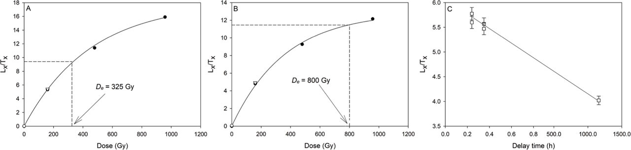
Representative sensitivity-corrected dose–response curves and dose estimates for sample 19088 for (A) IR50. and (B) pIRIR225. De was determined to be 325 Gy and 800 Gy, respectively. (C) Example of a g-value measurement of the IR50 signal on a single aliquot of sample 19088. The steep trend line suggests a significant fading of the IR50 signal.
To estimate the bleachability of the pIRIR225 signal from the Tatra samples and determine the residual dose, we performed a bleaching experiment on 18 aliquots of the feldspar sample 19087. The aliquots were exposed to artificial sunlight in a Hönle SOL2 solar simulator for different lengths of time: 1, 5, 20, 60 and 20,960 min (2 weeks). Subsequently, the relative bleaching of the IR50 and pIRIR225 signals was determined using the same protocol as for the De measurements. The dose recovery tests, anomalous fading and bleaching experiments are presented in the results.
. Dosimetry and Age Calculation
For the calculation of the ages, the average environmental dose rate since the time of deposition needs to be determined. Consideration must be taken of changing water content or nuclide leaching, which will affect the dose rate. In this study, the dose rate is assumed to have remained constant over time. The water content or soil moisture impact is related to the determination of dose rate and subsequent age estimation. Though important values for the age calculation, they are difficult to determine exactly since sedimentological, topographic and climatic conditions from the study area and their variation over time and depth must be accounted for (Rosenzweig and Porat, 2015).
To assess the sediment density and water content, the 100 cm3 soil sample rings were weighed in their natural state and after 24 h of saturation and 24 h at 105°C in an oven, respectively. The field water content (wcf) and the saturated water content (wcs) were calculated as mass% of the dry weight. The dry weight was also used to determine the sediment density.
An estimate of the average water content since the time of deposition is required for determination of the environmental dose rate. As no reliable data of the past water content in the foothills are available, the expected water content (wce) was estimated. This is carried out assuming that the wce is in between the wcf and the wcs, following the calculation method in Nelson and Rittenour (2015):
where pmax signifies an estimated percentage to calculate the maximum (saturated) water content and pmin represents the estimated minimum (field) water content percentage. For the Bee Pit samples, pmax was assumed depending on their depth below the estimated former ground surface of the gravel pit. The five samples located closest to the groundwater level at the bottom of the lower section (samples 19082–19086) were given a 0.7–0.9 range of pmax and a 0.1–0.3 range for pmin. The three samples located in the upper section of the Bee Pit were given a 0.4 pmax and a 0.6 pmin (Table S2). For the Velická dolina valley, the samples taken close to a new or old riverbed (samples 19098, 19105 and 19106) are presumed to have been saturated since deposition. The fluvial deposit near the riverbed is considered to have been somewhat drier, and for these samples (19101 and 19102), pmin is 0.1 and pmax is 0.9. For deposits positioned further away from the modern riverbed (sample 19100), pmin is 0.3 and pmax is 0.7. The samples with the highest elevation (samples 19093–19095) are assumed to have the lowest wce (Table S2).Ages for both quartz and feldspar were calculated using DRAC v1.2 dose rate and age calculator (Durcan et al., 2015). The ages were calculated based on the mean De and the sediment dose rate, considering sample- and site-specific information such as water content, depth and overburden density that affects the total environmental dose rate. For feldspar, a K-content of 12.5% was assumed (Huntley and Baril, 1997). Fading-corrected feldspar ages were calculated according to Huntley and Lamothe (2001) and using the function calc_FadingCorr in the R Luminescence-package (Kreutzer, 2020). Samples with negative g-values were not corrected for fading (Thiel et al., 2011a,b).
. Results
. Luminescence
. Quartz OSL
The IR/B tests showed that the quartz grains were contaminated with feldspar. The IR/B ratio was significant (>10%) for all but two samples (19094 and 19098B). For most samples, the ratio ranged from 16% to 46%; however, samples 19088 and 19105 displayed much higher values, ranging from 200 to 2000%. The samples were therefore measured with post-IR blue (Roberts and Wintle, 2001) or pulsed stimulation (Ankjærgaard et al., 2010) to reduce the influence of feldspar on the quartz OSL signal.
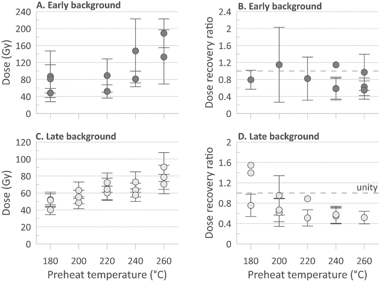
Using early background subtraction to enhance the fast signal component (Cunningham and Wallinga, 2010) led to large uncertainties in the dose determinations and higher rejection of aliquots. Doses and dose recovery ratios calculated with early background (Figs. 9A,B) nevertheless gave slightly more stable results with changing preheat temperature, at least until 220°C, than those calculated with late background (Figs. 9C,D). Late background doses show a trend towards higher mean doses with increasing temperature (Fig. 9C), while dose recovery ratios decrease with higher temperatures (Fig. 9D). Irrespective of integration interval and temperature, the measured dose severely underestimated the given dose for most aliquots (Figs. 9B,D; Table S2). There is considerable scatter between aliquots and large uncertainties for individual dose determinations, particularly for doses calculated with early background. This is likely mainly due to the weak signals; for natural doses, scatter related to incomplete bleaching may also contribute as discussed in the following text.
Fig 9.
Variation in equivalent dose and dose recovery ratio with temperature and signal integration intervals for sample 19082. (A) Preheat plateau (PHP) test where doses were calculated with early background subtraction (peak first 0.32 s, background next 0.32 s). All aliquots for 200° were rejected, (B) dose recovery ratios with corresponding calculation. (C) PHP test with late background subtraction for dose determination (peak first 0.8 s, background last 64 s). (D) Dose recovery ratios with corresponding calculation. The hatched line in B and D shows a dose recovery ratio of 1.0 (i.e. unity).
Analysis of the quartz OSL signal decay curves showed that the quartz signal is dim and that it had a weak fast signal component with significant contributions of medium and slow components (Fig. 10). The fast ratio calculations showed a low contribution of the fast component to the initial signals with average values of 1–4 (max 7). This is supported by the LM-OSL results (Fig. 11). Samples 19082 and 19095 exhibited the presence of five components, although with some distinctive differences. Whereas sample 19082 showed the presence of the slow1 component, this was not observable in the case of sample 19095. Moreover, only sample 19095 showed the presence of a medium component. Sample 19104 could be fitted with only three components: fast, slow1 and slow3 (Fig. 11C and Table 2). However, in none of the samples, the fast component was dominant. In contrast, for the Risø calibration quartz, only two components were observed: fast and slow4, where the fast component is clearly dominant in the initial signal. The calculated relative (σ) and absolute photoionisation cross-sections (σ (cm2)) for each of the detected components calculated from the fitted parameter ‘b’ are presented in Table 2.
Fig 10.
(A) Decay curve comparison between normalised OSL signals from quartz sample 19083 and Risø calibration quartz (Hansen et al., 2015) for the initial part of the stimulation. The decay curve of sample 19083 indicates a slow signal decay, which is not dominated by a fast component. (B) A similar comparison between non-normalised OSL signals shows the very dim signal of the quartz from the Biely Váh valley.
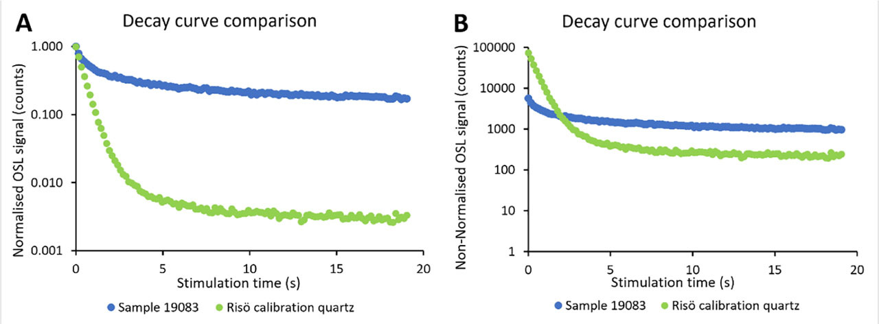
Fig 11.
LM-OSL curves for one aliquot each of samples: (A) 19082 (B) 19095 (C) 19104 and (D) Risø calibration quartz batch 123. It is notable that the presence of the fast component varies greatly between samples, but it is not dominant in any of the Tatra samples.
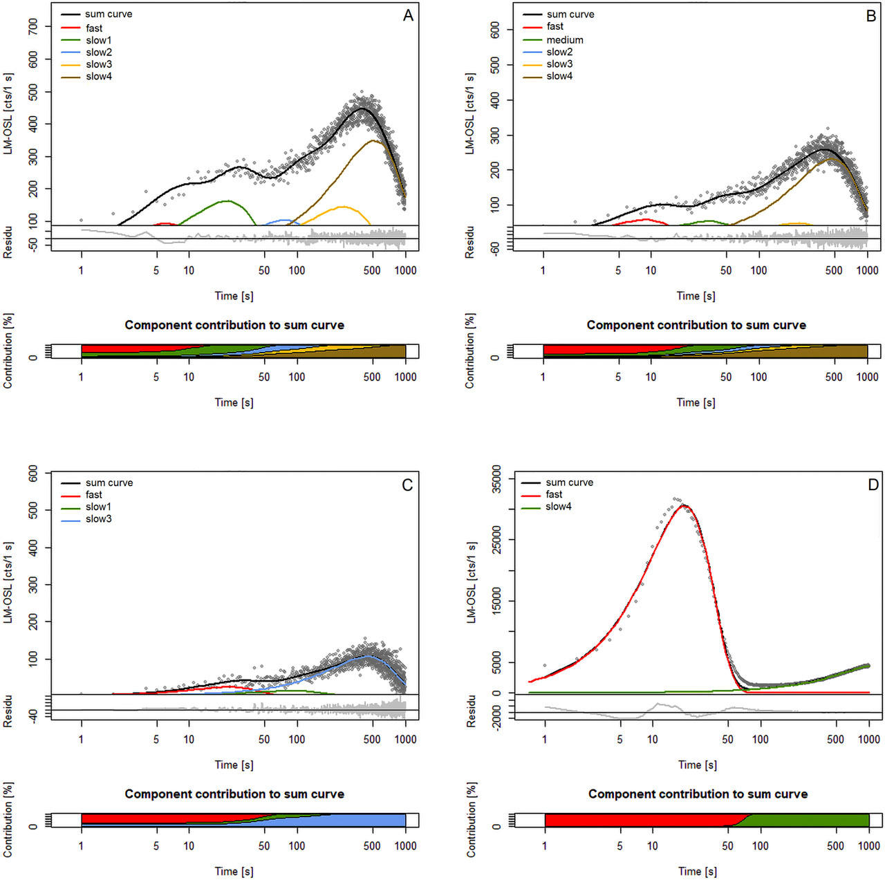
Table 2.
OSL parameters calculated from the quartz extracts using linear modulation compared to other values from literature.
| Sample | OSL component | Detraping probability (b) | Photoionisation cross-section (ϭ) | Relative Cross-section |
|---|---|---|---|---|
| 19082 | Fast | 22.4 ± 4.9 | 1.4 × 10⁻¹⁶ | 1 |
| Slow1 | 1.8 ± 0.2 | 1.2 × 10⁻¹⁷ | 0.09 | |
| Slow2 | 0.17 ± 0.003 | 1.1 × 10⁻¹⁸ | 0.01 | |
| Slow3 | 0.018 ± 0.004 | 1.1 × 10⁻¹⁹ | 0.001 | |
| Slow4 | 0.0004 ± 0.0003 | 2.5 × 10⁻²⁰ | 0.0002 | |
| 19095 | Fast | 9.6 ± 3.2 | 6.1 × 10⁻¹⁷ | 1 |
| Medium | 0.94 ± 0.1 | 6.0 × 10⁻¹⁸ | 0.1 | |
| Slow2 | 0.12 ± 0.008 | 7.8 × 10⁻¹⁹ | 0.01 | |
| Slow3 | 0.017 ± 0.0008 | 1.2 × 10⁻¹⁹ | 0.002 | |
| Slow4 | 0.004 ± 0.00009 | 2.9 × 10⁻²⁰ | 0.0006 | |
| 19104 | Fast | 1.6 ± 0.3 | 6.2 × 10⁻¹⁸ | 1 |
| Slow1 | 0.08 ± 0.04 | 5.0 × 10⁻¹⁹ | 0.05 | |
| Slow3 | 0.005 ± 0.0003 | 3.1 × 10⁻²⁰ | 0.003 | |
| Calib. quartz | Fast | 2.7 ± 0.09 | 1.6 × 10⁻¹⁷ | 1 |
| Slow4 | 0.0007 ± 0.00003 | 4.5 × 10⁻²¹ | 0.0003 | |
| Jain et al. (2003) | Fast | 2.5 ± 0.2 | 2.3 × 10⁻¹⁷ | 1 |
| Medium | 0.62 ± 0.05 | 5.6 × 10⁻¹⁸ | 0.2 | |
| Slow1 | 0.15 ± 0.03 | 1.3 × 10⁻¹⁸ | 0.06 | |
| Slow2 | 0.023 ± 0.005 | 2.1 × 10⁻¹⁹ | 0.01 | |
| Slow3 | 0.0022 ± 0.0002 | 2.1 × 10⁻²⁰ | 0.001 | |
| Slow4 | 0.00030 ± 0.00001 | 2.8 × 10⁻²¹ | 0.0001 | |
| Durcan and Duller (2011) | Fast | n.a. | 2.6 × 10⁻¹⁷ | 1 |
| Medium | n.a. | 4.3 × 10⁻¹⁸ | 0.16 | |
| Slow1 | n.a. | 1.1 × 10⁻¹⁸ | 0.04 | |
| Slow2 | n.a. | 3.0 × 10⁻¹⁹ | 0.01 | |
| Slow3 | n.a. | 3.4 × 10⁻²⁰ | 0.001 | |
| Slow4 | n.a. | 9.1 × 10⁻²¹ | 0.0003 | |
[i] The presented results represent the average values of two measured aliquots. For comparison, the values by Jain et al. (2003) and Durcan and Duller (2011) are shown.
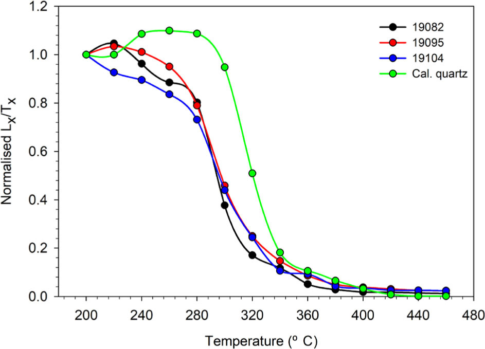
The results of the pulse annealing experiment are shown in Fig. 12. It is observable that the OSL signal from the quartz samples from the Tatra Mountains exhibits a sensible stability when compared to that from the Risø calibration quartz samples only up to 240 °C. This is especially evident at temperatures between 200 °C and 260 °C. A substantial decrease in the OSL signals for all the Tatra samples was observed after the temperature was raised above 260°C. For comparison, the signal of the calibration quartz remained stable even at a temperature of 300°C. Even though the OSL signal from the Risø calibration quartz commonly shows a better behaviour and increased stability when compared to natural samples, the results of the pulse annealing experiment suggest that quartz from the Tatra samples may suffer from thermal instability.
Fig 12.
Comparison of the thermal stability between the natural quartz extracts (samples 19082, 19095 and 19104) and the Risø 180–250 μm calibration quartz (batch 123).
Despite the unsuitable luminescence characteristics, a few dose estimates were made for some samples from the Bee Pit and the Velická dolina valley following the standard SAR protocol (Table 3). Differential OSL (Jain et al., 2005) did not improve the results (dose recovery ratio 1.22 ± 0.27, n = 6), dose estimates were still scattered (range 106 Gy to 392 Gy for 19082) and many aliquots failed the acceptance criteria (Table 3). Thus, we conclude that the quartz grains from the Tatra Mountains cannot be considered as a reliable dosimeter for luminescence dating. For this reason, the analysis shifted focus to feldspar.
Table 3.
OSL doses, dose rates and ages for the quartz samples.
. Feldspar IRSL: signals, doses and ages
The obtained environmental dose rate for feldspar ranges from 4.39 ± 0.26 Gy/ka to 1.78 ± 0.14 Gy/ka, with similar dose rate averages in the Biely Váh valley (3.34 ± 0.17 Gy/ka) and the Velická dolina valley (3.38 ± 0.22 Gy/ka) (Table 4).
Table 4.
Concentration of radioactive elements in the sampled sediments (from gamma spectrometry) and the dose rate from cosmic radiation to each sample (as calculated in DRAC v1.2 (Durcan et al., 2015)).
The measured K-feldspar IRSL signal was significantly brighter than quartz signal; moreover, the IRSL signal of pIRIR225 measurements was brighter than the IR50 signals. Fading measurements of the IR50 signal yielded g-values ranging from 1.6%/decade to 11.5%/decade, while for the pIRIR225, the g-values were lower, varying 0.1–3.3%/decade (Table 5). In addition, there is less variation in the g-values of the pIRIR225 than that in the g-values of IR50.
Table 5.
Results of the IR50 and pIRIR225 measurements: g-values, feldspar dose estimates, the number aliquots with De < 2D0 compared to the total number of accepted aliquots and the uncorrected and corrected ages.
| Sample No. | Unit / Site No. | g-value (%/decade) | De (Gy) | Accepted (De<2D0) / Total aliquots | Uncorrected age (ka) | Corrected age (ka) | |||||
|---|---|---|---|---|---|---|---|---|---|---|---|
| IR50 | pIRIR225 | IR50 | pIRIR225 | IR50 | pIRIR225 | IR50 | pIRIR225 | IR50 | pIRIR225 | ||
| 19082 | Unit 3 | 6.71 ± 0.1 | 2.23 ± 0.3 | 414 ± 15 | 868 ± 86 | 12(12)/12 | 12(1)/12 | 125 ± 7.8 | 261 ± 29 | 278 ± 18 | 326 ± 38 |
| 19083 | Unit 1B | 4.82 ± 0.7 | 1.56 ± 0.1 | 351 ± 14 | 844 ± 116 | 12(12)/12 | 12(1)/12 | 109 ± 7.2 | 263 ± 39 | 185 ± 28 | 308 ± 51 |
| 19084 | Unit 3 | 9.83 ± 0.2 | 2.84 ± 0.2 | 348 ± 14 | 741 ± 80 | 12(12)/12 | 12(2)/12 | 129 ± 8.7 | 275 ± 33 | 624 ± 82 | 368 ± 46 |
| 19085 | Unit 3 | 6.52 ± 0.1 | 1.66 ± 0.6 | 317 ± 11 | 760 ± 76 | 12(12)/12 | 12(1)/12 | 106 ± 6.8 | 254 ± 29 | 230 ± 16 | 300 ± 39 |
| 19086 | Unit 3 | 1.66 ± 0.2 | 0.09 ± 0.1 | 387 ± 16 | 812 ± 105 | 12(12)/12 | 12(0)/12 | 100 ± 7.3 | 210 ± 30 | 117 ± 8.7 | 212 ± 29 |
| 19087 | Unit 12 | 5.06 ± 0.3 | 1.48 ± 0.1 | 351 ± 13 | 788 ± 73 | 12(12)/12 | 12(2)/12 | 120 ± 7.6 | 269 ± 29 | 208 ± 16 | 311 ± 31 |
| 19088 | Unit 12 | 5.85 ± 0.2 | 0.81 ± 0.6 | 326 ± 11 | 776 ± 74 | 12(12)/12 | 12(1)/12 | 81 ± 4.9 | 193 ± 21 | 156 ± 12 | 208 ± 27 |
| 19089 | Unit 12 | 5.05 ± 0.02 | 1.99 ± 0.02 | 372 ± 14 | 850 ± 91 | 12(12)/12 | 12(2)/12 | 109 ± 6.6 | 249 ± 29 | 188 ± 11 | 304 ± 36 |
| 19090 | Unit 9 | 5.71 ± 0.4 | 2.16 ± 0.1 | 354 ± 13 | 763 ± 73 | 12(12)/12 | 12(1)/12 | 115 ± 7.8 | 248 ± 28 | 219 ± 22 | 308 ± 31 |
| 19091 | Unit 9 | 8.69 ± 1.1 | 0.37 ± 0.4 | 360 ± 13 | 710 ± 58 | 30(30)/30 | 30(8)/30 | 97.3 ± 5.7 | 192 ± 18 | 318 ± 185 | 199 ± 19 |
| 19092 | Unit 5 | 5.26 ± 0.3 | 0.70 ± 0.4 | 465 ± 20 | 949 ± 123 | 12(12)/12 | 12(2)/12 | 132 ± 8.6 | 269 ± 38 | 236 ± 19 | 287 ± 39 |
| 19093 | Site 1 | 8.01 ± 0.6 | 1.05 ± 0.3 | 338 ± 15 | 636 ± 64 | 12(12)/12 | 12(5)/12 | 79.5 ± 5.5 | 150 ± 17 | 219 ± 50 | 165 ± 19 |
| 19094 | Site 1 | 9.43 ± 0.5 | 3.04 ± 0.1 | 304 ± 14 | 611 ± 49 | 12(11)/15 | 12(7)/13 | 69.9 ± 5.2 | 139 ± 14 | 266 ± 105 | 188 ± 21 |
| 19095 | Site 1 | 4.83 ± 0.3 | 2.06 ± 0.2 | 325 ± 13 | 709 ± 85 | 12(12)/12 | 12(5)/13 | 86.1 ± 5.9 | 188 ± 25 | 145 ± 12 | 231 ± 29 |
| 19096 | Site 2 | 7.20 ± 0.6 | 1.52 ± 0.2 | 346 ± 14 | 770 ± 72 | 29(29)/30 | 29(9)/30 | 90.9 ± 6.1 | 202 ± 22 | 204.5 ± 34 | 234 ± 24 |
| 19097 | Site 2 | 7.25 ± 1.1 | −0.41 ± 0.1 | 330 ± 12 | 798 ± 88 | 12(12)/15 | 12(3)/18 | 96.7 ± 6.9 | 234 ± 30 | 234 ± 83 | * |
| 19098 | Site 3 | 8.61 ± 0.8 | 3.31 ± 0.2 | 134 ± 4.2 | 361 ± 22 | 12(12)/12 | 12(10)/12 | 38.5 ± 2.9 | 103 ± 9.5 | 116 ± 35 | 145 ± 14 |
| 19100 | Site 4 | 4.56 ± 0.6 | 1.43 ± 0.2 | 306 ± 15 | 839 ± 122 | 12(12)/12 | 12(2)/12 | 81.7 ± 6.1 | 224 ± 35 | 130 ± 14 | 257 ± 41 |
| 19101 | Site 5 | 11.49 ± 0.3 | 1.65 ± 0.2 | 131 ± 4.1 | 506 ± 37 | 12(12)/14 | 12(7)/12 | 37.7 ± 2.8 | 146 ± 14 | 307 ± 118 | 172 ± 17 |
| 19102 | Site 5 | 7.49 ± 0.9 | 2.60 ± 0.2 | 96.0 ± 3.1 | 387 ± 32 | 33(33)/33 | 33(22)/35 | 29.1 ± 2.0 | 117 ± 12 | 69 ± 15 | 152 ± 15 |
| 19105 | Site 6 | 10.77 ± 1.0 | 2.98 ± 0.3 | 31.5 ± 1.5 | 109 ± 7.0 | 12(12)/15 | 12(9)/18 | 17.7 ± 1.6 | 61.6 ± 6.3 | 79 ± 37 | 82 ± 10 |
| 19106 | Site 6 | 6.74 ± 0.04 | 1.64 ± 0.1 | 56.2 ± 1.9 | 183 ± 5.8 | 12(12)/15 | 12(9)/18 | 20.1 ± 1.6 | 65.4 ± 5.2 | 42 ± 3.5 | 77 ± 5.7 |
| 20026 | Site 2 | 5.42 ± 0.41 | 0.66 ± 0.25 | 453 ± 10 | 737 ± 47 | 5(5)/5 | 5(5)/5 | n/a | n/a | n/a | n/a |
| 20028 | Site 8 | 4.89 ± 0.83 | 0.88 ± 0.41 | 18.4 ± 3.9 | 55.6 ± 5.6 | 12(12)/12 | 12(12)/12 | 5.0 ± 1.1 | 15.0 ± 1.7 | 7.6 ± 2.0 | 16.1 ± 1.9 |
* Corrected age is not calculated due to a negative g-value. For dose rates, see Table 4.
The results of the dose recovery test showed that the best ratios (close to 1) are obtained from the pIRIR225 signal (Table S3), although most of them are in the lower 10% of the accepted range. With a few exceptions, the dose recovery ratios of the IR50 signal showed that the measured dose was underestimating the given dose. The average dose recovery ratios for all samples were 0.91 ± 0.03 (n = 7) for pIRIR225 and 0.87 ± 0.03 (n = 7) for IR50. The dose estimates of all the samples were in general also lower for IR50 than for pIRIR225. The IR50 signal generally shows a steady growth with dose, except for only one aliquot (sample 19094) that has a De value >2*D0 and thus is close to saturation (Table 5) (Wintle and Murray, 2006). However, the opposite is true for the pIRIR225 measurements, where most aliquots have De > 2*D0 (Table 5). Equivalent doses were nonetheless calculated for all aliquots, though in some cases with infinite errors. When comparing the Velická dolina valley to the Biely Váh valley, most aliquots of the samples from the Biely Váh valley from the pIRIR225 measurements have De > 2*D0, while in the Velická dolina valley, >50% of the aliquots with such high Des were observed only for samples 19093, 19095, 19097 and 19100 (Table 5). Representative dose–response curves for selected samples are shown in Figs. 13 and 14. The D0 value range from all the samples is 38-616 for IR50 and 5-462 for pIRIR225.
Fig 13.
(A) Dose–response curve and fading plot (inset) for the IR50 signal of sample 20026. Note that the signal does not display full saturation and fades significantly (mean g-value 5.4 ± 0.4%/decade for all aliquots). (B) Dose–response curve and fading plot (inset) for the pIRIR225 signal of sample 20026. The natural signal of this aliquot is close to saturation since the De > 2D0 (De = 765 ± 95 Gy; D0 = 289 ± 4 Gy) but not at saturation, and it still shows some fading in the laboratory (sample average g-value 0.66 ± 0.25%/decade).
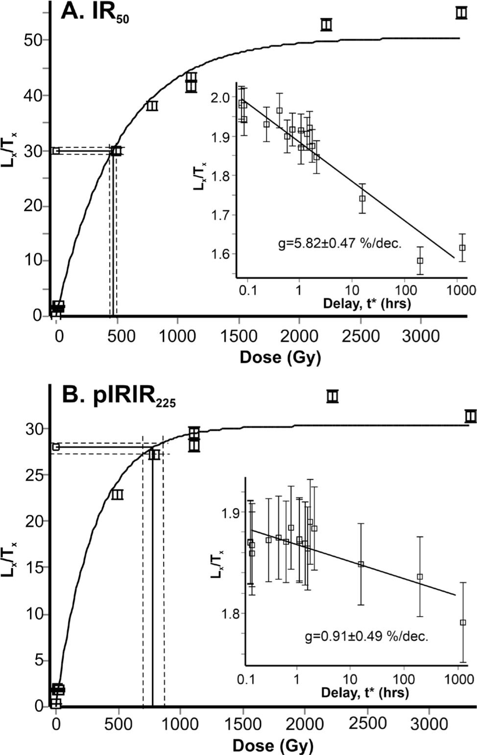
Fig 14.
Examples of growth curves for IR50 and pIRIR225 measurements for samples 19091 (A,B) and 19096 (C,D). For the aliquot of sample 19091, the De is closer to saturation for the pIRIR225 signal. Sample 19096 is not close to saturation for IR50 and pIRIR225 (i.e. De < 2*D0).
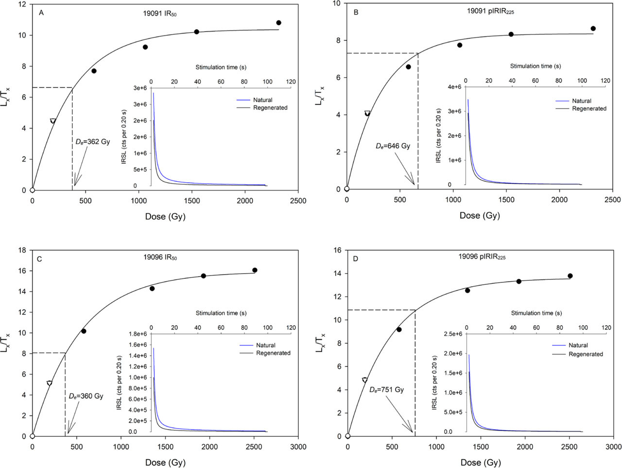
The doses for the non-modern samples range from 96.0 ± 3.1 Gy to 465 ± 20 Gy for IR50 and from 387 ± 32 to 949 ± 123 Gy for pIRIR225 (Table 5). The Des from the Velická dolina valley show a broader range from 96.0 ± 3.1 Gy (sample 19102) to 338 ± 15 Gy (sample 19093) for IR50 and for pIRIR225 from 387 ± 32 Gy (sample 19102) to 839 ± 122 Gy (sample 19100) than Des from the Biely Váh valley, where doses have a smaller range and are more consistent (Table 5). On average, the ratio of the pIRIR225: IR50 equivalent doses are around 2:1 or 3:1, except for sample 19102 with a ratio of 4:1 (Table 5). For the three samples of which more aliquots are measured (n = 29–33), probability plots are available (Fig. S4), where the statistical significance of skewness is tested. It can be seen that the three analysed samples are not significantly skewed (skewness < 1 × σ skewness (√(6/n)) (Bailey and Arnold, 2006; Arnold and Roberts, 2009).
The uncorrected ages from the Biely Váh valley range from 81 ± 4.9 ka to 132 ± 8.6 ka for IR50 and from 192 ± 18 ka to 275 ± 33 ka for the pIRIR225 signal. The overall lower uncorrected ages at the Velická dolina valley range from 17.7 ± 1.6 ka to 96.7 ± 6.9 ka for IR50 and from 61.6 ± 6.3 ka to 234 ± 30 ka for pIRIR225. The corrected ages for both valleys are between 1 and 1.7 times higher for pIRIR225 than the uncorrected ages, while for the IR50 ages, these values are between 1.2 and 8.1 times higher.
. Feldspar IRSL: bleaching
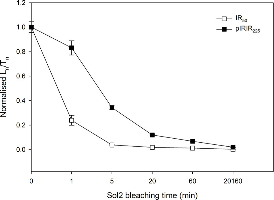
The results of the bleaching test of sample 19087 show that the IR50 signal bleaches at a significantly faster rate than the pIRIR225 signal (Fig. 15 and Table 6). After 1 min of bleaching, the normalised IR50 signal was reduced by 76% of the natural, while the equivalent pIRIR225 signal displayed a decrease of only 17%. Following a 5-min bleach this discrepancy becomes even more evident: the IR50 signal displayed a decrease of 96% when compared to the natural, whereas the pIRIR225 signal retained 34% of its initial value.
Fig 15.
Bleaching rate of sample 19087 showing the signal or dose (Gy) plotted against exposure time in a logarithmic scale for both IR50 and pIRIR225.
Samples 19105 and 19106 are modern analogues, taken to evaluate bleaching and residual doses in the present-day fluvial environment. Sample 19105 was taken at the surface and 19106 was taken 3 cm below. Most aliquots from both samples do show signals and thus not a zero dose. Instead, the De of sample 19105 is 31.5 ± 1.5 Gy when stimulated with IR50 and 109 ± 7.0 Gy for pIRIR225. For sample 19106, the dose is 56.2 ± 1.9 Gy for IR50 and 183 ± 5.8 Gy for pIRIR225 (Table 5).
. Discussion
. Quartz OSL
Even though several variations of dose estimate measurements were performed on the quartz samples, post-IR blue OSL (Roberts and Wintle, 2001), pulsed OSL (Ankjærgaard et al., 2010) and differential OSL (Jain et al., 2005), none of them yielded reliable results. This issue is most likely related to a combination of unfavourable luminescence characteristics such as dim signal, thermal instability, weak fast signal component and/or unstable signal components. The pulse annealing experiments suggest that quartz from the Tatra Mountains is unstable and the OSL signal is most likely affected by thermal fading (Fig. 12). Moreover, the LM–OSL measurements revealed large discrepancies in the quartz behaviour of the analysed samples (Fig. 11). While for samples 19082 and 19085, five components were detected, the distant modern analogue sample (19104) displayed a three-component signal (Table 2). At the same time, all of the investigated samples lacked an OSL signal with a dominant fast component, which is considered a most unfavourable behaviour for luminescence dating. Although the relative cross sections show a generally good agreement with previous studies, all absolute σ values are considerably higher, varying between a factor of 3 and 10. As suggested by Bulur et al. (2002) and Choi et al. (2006), it appears that the number of integral OSL components and their properties can exhibit large variations from sample to sample, regardless of the same sampling site, which seems to be the case for quartz from the Tatra Mountains. At present, we are uncertain about the reason for such discrepancy between the investigated samples. One explanation may be that the samples originate from diverse primary sources which might have caused the difference in the signal characteristics (Perić et al., 2021).
The decay curve shape (Fig. 10A) and low fast ratios lead to low-resolution dose determination and a high percentage of rejected aliquots therefore also a reduction in the quantity of De values (Trauerstein et al., 2017) and problems of true depositional age estimation (Steffen et al., 2009).
The obtained quartz ages ranged from 40–60 ka (Table 3), but showed unreliable results, which could have multiple reasons, among which an important factor is that the sediment samples in this study have doses higher than 200 Gy, which is usually beyond the reliable natural dose range for quartz luminescence dating (Buylaert et al., 2012; Avram et al., 2020; Perić et al., 2021).
. Feldspar IRSL
. Bleaching of IR50 and pIRIR225 signals
In this study, it was observed that feldspar is more favourable for luminescence dating than quartz in terms of signal characteristics. However, there are some features of the feldspar that need to be considered when assessing the results, such as bleaching, fading and saturation.
A prerequisite for accurate luminescence dating is that the analysed sediment was effectively bleached at the time of deposition (Murray et al., 2012). It is therefore important to identify any incompletely bleached grains or samples. In this study, we have used modern analogues (Alexanderson and Murray, 2012; Kars et al., 2014), experimental bleaching tests (sample 19087) (Lowick et al., 2012; Murray et al., 2012; Kars et al., 2014; Arnold et al., 2015), comparisons between different minerals, signals and, to some extent, dose distributions (Colarossi et al., 2015; Gliganic et al., 2017).
The modern analogues (sample 19105 and 19106) are presumed to have been deposited when the water level of the Velický potok river was at least ∼25 cm higher than at the time of sampling. Given the proximity to the present riverbed and the appearance of the site, this high-flow event is believed to be recent, perhaps during spring snowmelt or a heavy rain within the last (few) years (Kotarba, 2007). The sediment is therefore presumed to be young and should theoretically contain a dose close to zero. However, the modern analogue samples 19105 and 19106 reveal relatively high natural IR50 and pIRIR225 De values (Table 5). This implies that the feldspar samples have not been completely bleached in the present depositional environment. This is particularly evident in the case of the pIRIR225 signal, where a ∼60 Gy De value was observed. The doses are higher than other high-temperature pIRIR doses from modern analogues from similar settings, which range from ∼2 to ∼50 Gy (Alexanderson and Murray, 2012; Kars et al., 2014; Arnold et al., 2019). The apparent poor bleaching is likely due to short transport distance and turbid water in the Velický potok river (cf. Gliganic et al., 2017), particularly if the deposits derive from a flash flood. The same can be assumed for other material of the same grain size, transport and deposition mode in the southern foothills of the Tatras. For some of our older samples (19082, 19083 and 19084), the amount of received sunlight was undoubtedly even lower than the modern fluvial stream samples as they are classified as mass movements, debris flows and hyperconcentrated flows. This makes the modern samples less of an analogue for the other sites, although they still highlight the level of incomplete bleaching and indicate a risk of age overestimation for several of our samples.
Table 6.
Results of the SOL2 bleaching experiment for sample 19087.
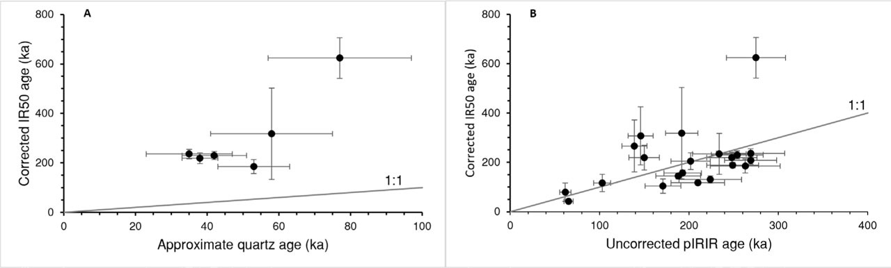
One of the most used methods to determine whether the pIRIR signal is likely to have been fully reset is the comparison with quartz signals or other IR signals that have different sensitivities to daylight. It is known that the IR50 signal bleaches more rapidly in sunlight than IR signals stimulated at elevated temperatures (Thomsen et al., 2008), as also shown in our bleaching experiment (Fig. 15). The slower resetting of the pIRIR225 signal is possibly linked to the various used preheat temperatures, probably through a thermal transfer process (Buylaert et al., 2012). However, even though the pIRIR225 shows a much slower bleaching rate than the corresponding IR50 signal, it is obvious that an efficient resetting is possible in a natural environment. In an effectively bleached sample, quartz ages and fading corrected IR50 and pIRIR225 ages should display a good agreement, assuming that there are no other problems with the signals (like dim signal and weak fast component). For all the six samples where quartz and feldspar ages were calculated (Tables 3 and 4), quartz ages are considerably younger than the corresponding feldspar ages (Fig. 16A). However, due to the quartz luminescence characteristics, the quartz ages may be underestimated and the comparison with feldspar ages not reliable. For most samples, the pattern between the two feldspar signals is as expected, with corrected IR50 ages similar to or lower than the uncorrected pIRIR225 ages, but for four samples, the corrected IR50 ages are outside 1 σ higher than the uncorrected pIRIR225 (Fig. 16B). This discrepancy could be due to the added uncertainties caused by a relatively large fading correction for the IR50 signal. From a bleaching perspective, samples with the same or similar age for uncorrected pIRIR225 and corrected IR50 are considered more reliable.
Fig 16.
Comparison between quartz and feldspar ages. (A) Approximate quartz ages, based on 3 aliquots per sample, are all much lower than the fading corrected IR50 ages. (B) Feldspar-corrected IR50 ages are mostly of the same order as the uncorrected pIRIR225 ages, with some exceptions.
Subtracting the residual dose could potentially correct for any dose (age) overestimation produced by an unbleachable dose. However, when the residual values (Table S3) are subtracted from modern analogue samples 19105 and 19106 (Table 5), the dose is still not close to zero neither for IR50 nor pIRIR225. Given the negligible residual values for the De calculations of the older samples, they were not subtracted, as suggested by Li et al. (2013) and Kars et al. (2014).
The recent transportation of sediment from the Tatra Mountains by a river provides better bleaching conditions than the sediment transportation in a glacial environment characterised by mass movements and hypercontracted flows. One could argue, therefore, that the modern analogues would be a better measure than the bleaching experiment residual for the effect of incomplete bleaching for the old sediments and that subtracting a dose of that magnitude from each determined De would give a truer age. When the average of the pIRIR225 doses (146 ± 5.8 Gy) of the modern analogues (19105 and 19106) is subtracted from the other samples and the ages are calculated, the uncorrected pIRIR225 ages are, on average, 44 ± 3 ka and 42 ± 1.5 ka younger for the Bee Pit and the Velická dolina valleys, respectively (the difference ranges from 33 ka to 65 ka for both areas). These ages would be outside 1 σ (error) of the original ages for all samples. However, from a sedimentological perspective, as discussed earlier, even the modern analogues may underestimate the remaining (unbleached) dose for some of the older deposits.
It is in this context interesting to note that the sampled moraine (Site 8, sample 20026) seems to consist of effectively bleached material. At least its age (15.0 ± 1.1 ka, uncorrected pIRIR225) agrees with cosmogenic exposure ages from a similarly situated moraine in a nearby valley (20.0 ± 1.0–16.7 ± 0.7 ka; Makos et al., 2014). This may indicate that much of the moraine derives from supraglacial material, which was bleached on the glacier surface prior to deposition (Zeng et al., 2016).
To evaluate potential incomplete bleaching for the older (higher dose) sediments, we can also observe dose distributions and compare the ages within units. The dose distributions of samples 19091, 19096 and 190102 (Fig. S4) show that these three samples (n = ∼30) are normally distributed. For all of them (except for sample 19091), the pIRIR225 Des are slightly positively skewed but not significantly so. In cases where incomplete bleaching is present, usually a higher positive skewness or tail of high doses is expected. However, that does not seem to be the case for these samples.
The number of samples from the Bee Pit and the GYW also allowed us to compare ages from the same units, which should depict a similar age. Though the numerical uncertainty of each age is relatively large (12% on average), there is a scatter of ages within units, and not all sample ages from one and the same unit overlap within 2σ (Figs. 3 and 5; Table 5). Furthermore, the variation in age between the samples from the same site or unit is higher in the IR50 measurements than the uncorrected pIRIR225 ages (cf. Arnold et al., 2015). Scattered values would be expected if the sampled sediments had different transport and light exposure histories, which would result in an irregular bleaching of the grains. In that case, the youngest age from each unit would originate from the best bleached sediment within that unit and thus represent the most accurate age, though it may still not be an overestimation. This is under the assumption that there is no significant small-scale dose rate heterogeneity, which also could cause age variability within a unit (Jankowski and Jacobs, 2018; Smedley et al., 2020). However, we do not have the data to assess this.
In terms of bleaching, we conclude that most of our samples do suffer from incomplete signal resetting and thus overestimate the true age. Therefore, the calculated ages should, in this case, be considered as maximum ages. The degree of age overestimation varies, though, and the youngest age in a specific unit may be considered the age closest to the true age of that unit.
. Fading and saturation
Anomalous fading could be responsible for underestimating the equivalent doses and making the ages seem younger than they truly are, hampering their accuracy (Banerjee et al., 2001; Thiel et al., 2011a). The uncorrected IR50 doses are consistently lower than their pIRIR225 counterparts from the same sample (Table 5). This is expected because the pIRIR225 signal is a measurement that minimises fading, making the age closer to the actual age of deposition, while the IR50 signal fades significantly (Buylaert et al., 2009). As expected, our samples show higher fading rates for the IR50 (4.6–11.5%/decade) than the pIRIR225 signals (0.09–3.3%/decade; Table 5). For the pIRIR225 signal, all g-values, except for samples 19094 and 19098, are lower than 3%/decade, which would correspond to an age correction of ∼35–40% for these samples, based on the function of Huntley and Lamothe (2001).
The g-values of both the IR50 and the pIRIR225 signals are higher than those of some other studies, where the IR50 g-value generally ranges from 1 to 4%/decade, while for the pIRIR225 signal, the g-value varies from 0 to 1.5%/decade (e.g. Thomsen et al., 2008; Thiel et al., 2011a,b). Usually, when the g-values of the pIRIR225 signal are <1–1.5%, they are difficult to assess (Roberts, 2012). Consequently, it was suggested in numerous studies (e.g. Buylaert et al., 2012, 2013; Roberts, 2012) that the application of the uncorrected pIRIR225 ages would be preferable.
The overall high g-values of the IR50 and some high outliers of pIRIR225 g-values also resulted in ages with higher errors as the large fading correction made the age more uncertain. Ideally, the corrected IR50 and the uncorrected pIRIR225 ages should yield similar results, given that the pIRIR225 minimises the fading effect (Table 5 and Fig. 14B) (Buylaert et al., 2009). In this case, nine samples overlap within 1 σ (19082, 19085, 19090, 19091, 19092, 19096, 19097, 19098 and 19105) and another eight within 2 σ (19083, 19087, 19088, 19089, 19094, 19095, 19101 and 19102) (Table 5 and Fig. 17) The younger IR50 ages (in comparison to the pIRIR225 ages) could be a result of the faster bleaching of the IR50 signal compared to the pIRIR225 signal, as discussed earlier. The same discrepancy is found for some of the corrected pIRIR225 ages (Table 5). For these reasons, we choose the fading uncorrected pIRIR225 ages as the preferred ones in this study.
Fig 17.
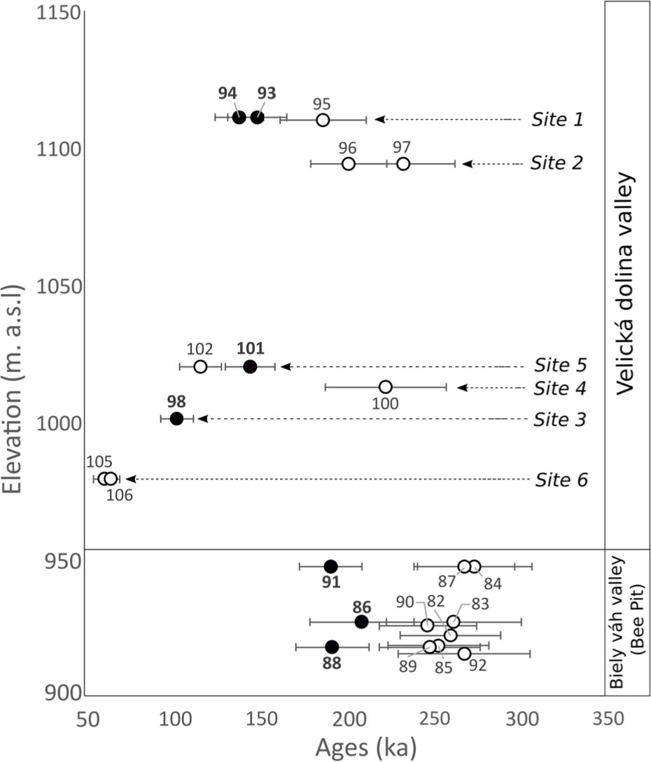
Relation of uncorrected ages of the pIRIR225 (ka) on the x-axis vs. elevation of the samples in the outcrops on the y-axis. Preferred ages per site or unit are black. Note that the Velická dolina valley and the Biely Váh valley are two different areas in the southern foothills of the Tatra Mountains and are not subsequent geological strata as the figure might imply.
Another important characteristic of these feldspar samples is saturation. Wintle and Murray (2006) stated that if the samples have doses >2*D0 and lie in the dose region where the laboratory growth curve starts to flatten out, the ages could potentially be older than is displayed and the De represents a minimum age. Most of the measured aliquots from our samples displayed De values >2D0 (i.e. close to saturation) for pIRIR225. This indicates that fading is negligible for the pIRIR225 signal (Table 5) (Thiel et al., 2011a,b) and supports favouring the ages obtained from the uncorrected pIRIR225 signal. However, some fading occurs even for the pIRIR signal, as is indicated by our boulder sample (20026), which should be in field saturation; but the Ln/Tn still intersects the growth curve (Fig. 13). The aliquots that had >2*D0 and their equivalent doses are included in our age calculations (Murray et al., 2014). From the perspective of saturation, the pIRIR225 ages should be considered minimum ages, but the samples with fewer aliquots close to saturation could be regarded as more likely to be near the true age. Samples that have >50% aliquots with De < 2D0 for pIRIR225 are 19094, 19098, 19101 and 19102 (Table 5), which could be considered more reliable.
. Determination of the ages
The process of estimating and evaluating the ages needs to consider all the features that have been discussed earlier, such as insufficient bleaching, saturation and number of aliquots, as well as the environmental dose rates, all of which have a clear impact on the final result. Several of the samples are not ideal in this context as they suffer from incomplete bleaching and/or have high doses close to saturation. Here, we will use the postulations outlined in Section 6.2 to evaluate the ages and conclude which ones were found the most reliable.
Based on the relatively low fading rates and the increased uncertainty that would be created when correcting for fading, we conclude that the uncorrected pIRIR225 signals would present the most reliable ones for age calculation of the different luminescence techniques applied.
The environmental dose rates are fairly consistent in the two study areas, and the largest uncertainties related to that are estimation of average water content since the time of deposition and, for some samples, heterogeneous sediments, for example, proximity to clasts. To evaluate the effect of changing water content, we calculated ages for three of the samples with different water content: completely dry (wc = 0%) and oversaturated (wc = 50%), see Table S5. The ‘dry’ and ‘wet’ ages are just outside 2σ of each other, so the age change is significant. However, we consider both a completely dry and an oversaturated setting highly unlikely, and the real possible range of water content to be less than 50%; hence, any age change related to water content smaller and not significant, particularly given the other uncertainties of the ages. Proximity of clasts to samples is mainly a concern for the dose rates for samples from the GYW, where sediments were clast-rich. To some extent, the clasts were included in the sediment dose rate measurement, and the clast lithology was similar to that of at least the gravel particles in the sediment. Hence, we do not regard the sediment heterogeneity as a significant problem for the sample dose rate.
Considering the larger stratigraphic context, a trend of age decrease from lower to upper units at the two main sites was expected: the Bee Pit and the GYW (Sites 1 and 2). Based on the arguments previously discussed, we can identify the Bee Pit samples that are likely to be most reliable and compare those stratigraphically. Sample 19091 (192 ± 18 ka) from unit B9 would, in this case, present the most reliable one, being the youngest age of its unit and having most aliquots and the least De scatter. Samples 19088 (unit B12; 193 ± 21 ka) and 19086 (unit B3; 210 ± 30 ka) are likewise the youngest in their respective units and from a bleaching perspective could be considered closest to the true age. The ages of these three samples, taken from deposits that span >30 m thickness, still overlap. However, the age range is smaller and centres around 200 ka. Assuming the ages are accurate, this would imply a very rapid sedimentation and build-up of these deposits. This scenario is not unfeasible, considering the type of deposit and that the apparent duration is still several tens of thousands of years and thus potentially encompassing several depositional periods. However, more than 50% of the samples yielded De values above 2*D0 (Table 5) with a dose magnitude larger than the corresponding quartz doses (Table 3), which indicates that these ages may still represent maximum ages.
At the GYW, the pIRIR225 ages from the upper units (139–188 ka; samples 19093–19095 from unit Y3 at Site 1) are younger than those of the samples from the lower unit at Site 2 (202–234 ka; samples 19096 and 19097), though the large errors lead to a partial overlap (Fig. 17). For unit Y3 (Site 1), sample 19093 (150 ± 17 ka) would represent the most reliable in terms of bleaching, while sample 19094 (139 ± 14 ka) would be favourable in terms of saturation (>50% below 2xD0). We find that these two samples provide the best age determination of unit Y3 and reject the older sample 19095 (188 ± 25). For Site 2, the ages from both samples 19096 and 19097 are supported by their agreement with the fading corrected IR50 ages (Table 5). Sample 19096 (202 ± 22 ka) is preferred based on the number of measured aliquots. The preferred ages at Sites 1 and 2 do not overlap and separate the depositional events into two different time periods, ∼140–150 ka and ∼200 ka, respectively.
Most of the measured aliquots for sample 19098 displayed De values <2*D0 (Table 5). The agreement of pIRIR225 and corrected IR50 ages (Table 5) indicate that these signals were bleached to a similar degree, though given the context of Site 3 (flood deposit), the age (103 ± 10 ka) is likely an overestimation of the true age. Sample 19100, taken from a mass movement, consists of a mix of sediment from several stratigraphic layers, resulting in inconsistent De values, and a maximum age (224 ± 35 ka). Samples 19101 and 19102, from Site 5, do not overlap within uncertainty (Fig. 17). Based on the glacifluvial deposition, we favour the youngest age of sample 19102 (117 ± 12), which also has the most measured aliquots (33) with the majority displaying De values <2*D0. Based on the calculated age, here, we argue that this terrace deposit (Site 5) was pasted onto the GYW at a later stage, making the lowermost part of the site younger than the deposits at higher elevation, GYW Sites 1 and 2.
. Chronology of the Southern Foothills
The Quaternary deposits on the southern Tatra foreland have been studied since the beginning of the nineteenth century (e.g. Zejszner, 1856); however, their chronostratigraphy is poorly established due to the lack of numerical dating. Although the chronology of the Tatra Mountains was significantly improved in the last two decades (e.g. Makos et al., 2014; Engel et al., 2015; Kłapyta et al., 2016; Pánek et al., 2016; Engel et al., 2017), the age of the ice-related sediments on the Tatra's foreland is still ambiguous. The sediment calibre and depositional structures indicate that the sampled sediments were deposited by a wide range of sedimentary processes in a proglacial environment. During the analysis of the data, the sediments proved to have a complex age determination (Sections 6.1 and 6.2), which produced uncertainties in the calculation of their ages. We attempted a comparison between glaciation cycles and deposition time frame of our samples, though it is hampered by the large uncertainties of the ages.
It is noteworthy that the ages from the Bee Pit (210 ± 30 ka) seem to largely agree with the age from Site 2, sample 19096 at the Velická dolina valley (202 ± 22 ka) where both are interpreted as hyperconcentrated flows. Other ages that overlap within 2 sigma are the ages from sample Site 1 (150 ± 17 ka and 139 ± 14 ka) and 5 (117 ± 12 ka), both from the GYW where Site 1 represents the top section and Site 5 is deposited and pasted on the lower layer(s). Assuming these sites truly formed during the same period, this could suggest a fast incision rate of the Velická dolina valley, where Site 1 is likely deposited before the incision and Site 5 after.
The preferred ages from the Bee Pit, which range between 193 ± 21 ka and 210 ± 30 ka (MIS 6–7), were compared with the established glaciations in the Tatras, which in the published literature have been correlated and named according to the Alpine system (i.e. Mindel, Riss, Würm). The Bee Pit ages coincide primarily with deposits dated between 228 ± 44 ka and 263 ± 36 ka on the Polish side of the Tatras and correlated to the Riss glaciation according to Lindner et al. (1993), that is, the later part of the Middle Pleistocene. Moreover, the presence of the glacier ice and its corresponding glaciofluvial deposits during the Riss glaciation have been identified in the southern foreland of the Tatra Mountains, in the vicinity of Štrbské Pleso, where the moraines are found in contact with glaciofluvial deposits (Lindner et al., 2003). This places the glacier extent quite close to the study area in comparison to the Riss II glaciation.
At the GYW in the Velická dolina valley, the oldest reliable (Section 6.2.3) age of 202 ± 22 ka is sampled in unit YN1 (sample 19096) and the youngest age of 139 ± 14 ka is sampled in unit YS3 (sample 19094). Sample 19096 was recovered from the hyperconcentrated flow deposit that suggests a high energy depositional environment most likely during the Riss I glaciation (MIS 6–7). On the one hand, the amount of suspended sediment in the meltwater increases in a colder climate due to the erosion caused by the glacier, supporting the interpretation of the deposition during a glacial period. On the other hand, such settings can also occur in transition phases from cold to warm periods that are typical of increased meltwater river discharge (e.g. Olszak et al., 2019). The upper deposit from the GYW (Site 1; Fig. 4 (YS3)) correlates to the Riss II glaciation (between MIS 5–6). The terrace deposited at Site 5 has an age of 117 ± 12 ka (sample 19102), which is older than the oldest dated deposit of the Late Pleistocene Würm glaciation (89 ± 13 ka) (Lindner et al., 2003). Based on this, we argue that the terrace sediments were deposited before the Würm glaciation, possibly during the Late Riss II (MIS 5).
The moraine in the upper part of the Velická dolina valley (Site 8) was deposited during the last deglaciation, ∼15 ka ago, similar to that in other valleys in the Tatra Mountains (Engel et al., 2015; Makos et al., 2014, 2016).
. Conclusions
An abandoned gravel pit in the Biely Váh valley and several sites in the Velická dolina valley in the southern foothills of the High Tatra Mountains were dated by luminescence dating. The interpretations and discussion of the data allowed to draw the following conclusions.
The luminescence dating analysis for the 27 samples of the study area presented certain challenges. The OSL quartz analysis did not yield reliable results, even though several measurement alternatives were applied (standard SAR protocol, pulsed stimulation, differential OSL and LM-OSL). The conclusion was that quartz was contaminated with feldspar and thermally instable, and had a dim signal, a weak fast signal component and/or unstable signal component. Pulse annealing supports the assumption that quartz from the Tatra Mountains is unstable and that the OSL signal is influenced by thermal fading.
The signal of the feldspar displayed in general a brighter signal and presented a better option to determine the ages of our samples. Four ages were calculated for each sample using both IR50 and pIRIR225 signals, with and without correction for anomalous fading. The g-values for the pIRIR225 were relatively low (<1–3.3%/decade), and the uncorrected pIRIR225 ages were selected as the ages that estimate the most reliable time of deposition. These ages indicate that the sediments in the Biely váh and Velická dolina valleys were deposited during the later part of the Middle Pleistocene and the early Late Pleistocene. An exception is a moraine in the upper Velická dolina valley, which was dated to the last deglaciation (∼15 ka). However, for most of the samples, incomplete bleaching and high doses close to saturation lead to large uncertainties for the ages.
Given the nature of the sediments and complex transport history, it is recommended to attempt to sample the sediments further downstream in the Biely váh and Velická dolina valleys. A longer distance from the source could possibly provide a longer bleaching time for the sediments. Likewise, for further studies in the area, it is suggested to test other dating methods that would be less affected by the unfavourable luminescence characteristic of these sediments due to their depositional environment.