
. INTRODUCTION
Calcium carbonate, with the chemical formula CaCO3, stands among the most widespread minerals of earth's crust. The importance of dating calcium carbonate based formations for setting age limits has been well demonstrated by both the uranium series disequilibrium method as well as Electron Paramagnetic Resonance (EPR) techniques. As far as luminescence techniques are concerned, Wintle (1977, 1978) has undertaken some of the initial work to assess whether the TL signal from calcite could be used to date geologically relevant samples. The reader may also refer to McDougal (1968) for a review of earlier achievements on this related topic. Due to the problematic properties, or even the lack, of optically stimulated luminescence (OSL) signal, thermoluminescence (TL) stands as the only luminescence technique available for dating applications for these formations.
Despite the numerous reports dealing with the EPR dating applications of calcium carbonates (for example Ikeya, 1993 and references therein), a limited number of papers deal with the corresponding luminescence applications of this mineral within the last 35 years (Debenham, 1983; Debenham and Aitken, 1984; Down et al., 1985; Ninagawa, 1987; Ninagawa et al., 1988, 1992; Liritzis, 1989; 2010; 2011; Duller et al., 2009; Stirling et al., 2014; Polymeris et al., 2016), both successful and unsuccessful. Throughout this aforementioned literature, the TL properties of various types of CaCO3 samples have been reported and the ages were in most cases lower than 500 ka. The present study provides methodological aspects on the ED estimation using the multiple-aliquot additive-dose procedure in the TL of calcium carbonate samples. Two different alternative approaches were adopted, namely a TL peak resolved analysis following deconvolution and the plateau method without deconvolution. Four different samples from the Quaternary were studied.
. MATERIALS AND METHODS
Apparatus
All luminescence measurements were conducted using a commercial Risø TL/OSL system (model TL/OSL-DA-20), equipped with blue LEDs (470 nm, FWHM 20 nm) and a 90Sr/90Y beta particle source, delivering a nominal dose rate of 0.1083 Gy/s. An EMI 9235QB photo-multiplier tube was used for the detection of all luminescence signals. For the cases of the few OSL and TA – OSL measurements, a Hoya (U-340) filter was used for light detection (340 nm, FWHM 80nm) while for all TL measurements only a BG-39 glass filter was used to restrict the wavelengths detected, similar to the studies of Duller et al., (2009) as well as of Polymeris et al. (2016). This filter has a transmission window that ranges from 350 to 600 nm and it was used for all TL measurements. All heatings and TL measurements were performed in a nitrogen atmosphere using a low constant heating rate of 2°C/s in order to avoid significant temperature lag (Kitis et al., 2015); the samples were heated up to the maximum temperature of 500°C. All luminescence measurements were conducted at the Institute of Nuclear Sciences of Ankara University.
For the structural characterization of the materials, the X-ray powder diffraction (XRPD) technique was applied; the minerals were analyzed to verify their crystalline structure using a Philips diffractometer with monochromatic CuKa (λ = 0.15406 nm) radiation. For a description of the elemental-chemical composition of the samples, Polarized Energy Dispersive X-ray fluorescence (XRF) analysis was performed using an X-ray Fluorescence spectrometer Spectro XLAB-2000. Both PXRD and XRF measurements and analysis were performed at the Earth Sciences Application and Research Center of Ankara University (YEBIM).
Materials and treatment
In this work, four different travertine samples were collected from the Bor district of Niğde city, Central Anatolia, Turkey. Travertine deposits are the product of calcium carbonate precipitation under cool water (Ford and Pedley, 1996). The thickness of the deposits differs between 15 and 25 meters. These deposits are considered belonging to the Quaternary, based on indirect proxies as well as preliminary luminescence dating results (Öztürk et al., 2018). The Southern part of study area was bordered with Bor Segment of Tuzgölü (Saltlake) Fault Zone, Turkey.
Based on Electron dispersion X-ray (EDX) spectroscopy, all samples contain predominantly Ca (38.85%), O (37.87%), while to a lesser extent C (21.03%); all percentage values indicate average values over all samples of the present study. This observation is in excellent agreement with the results of X-ray powder diffraction (XRPD) patterns, indicating the presence of the phase of CaCO3 solely. The sample codes as well as the concentration of each main element are presented in Table 1 for each sample. Typically, travertines are formed where cool carbonate supersaturated freshwater degasses and this is where karst water reaches the surface. Thus, various impurities are expected into the otherwise clean CaCO3 precipitate. Table 1 also presents the XRF results for other available elements as well, including K, Na, Fe, Mg, Mn, Si, Al, Ti and Cl. In some cases, the corresponding concentrations are below the detection limit of the PXRD technique.
Table 1
Content of main elements. The detection limit for the (%) concentration is 0.01%. BDL=Below Detection Limits.
Before luminescence measurements, treatments and preparation were under-taken in subdued red filtered light conditions. An almost 1 cm thick, outer layer was removed from each sample in the laboratory, to eliminate the light-subjected parts of the samples. Finally, grains with dimensions in the range 4–12 μm were extracted by gently crushing in an agate pestle and mortar, then suspended in acetone and finally precipitated onto 1 cm diameter aluminum discs (Fleming, 1979). As PXRD indicated the presence of solely CaCO3, no further chemical procedure was applied.
Methods of analysis
For the equivalent dose estimation the multiple aliquot additive dose procedure (MAAD) in TL was applied. A detailed description of the procedure can be found in Aitken (1985; 1998), Wagner (1998) and Liritzis et al. (2013). Mass reproducibility for all discs-aliquots was kept within ±3%. The additive doses applied were 0 (NTL), 150, 300, 450, 600 and 900 Gy. Four fresh aliquots were used for each additive dose. The equivalent dose (ED) was calculated using two different approaches. For the first approach, the ED was calculated using the plateau method (Aitken, 1985; Wagner, 1998) according to the following equation (Liritzis, 2010; Liritzis et al., 2015; Aidona et al., 2018):
where NTL is the natural TL glow curves, (NTL +βi) denotes the glow curves after the beta doses were added on top of the natural signal and βi the corresponding administered beta dose in units of Gy. Si denotes the slope of the (linear) fitting of the dose response curve and is defined according to the following equation (Polymeris et al., 2012; Liritzis et al., 2015):Eqs. 2.1 and 2.2 were applied to the entire NTL and NTL +βi glow curves. Since all TL curves were measured using 500 data points and heating rate of 1°C/s up to a maximum temperature of 500°C, the preceding calculations take place for each data point of the glow curves. Eventually Eq. 2.2 gives five different curves, each one corresponding to one among the additive doses applied with each data point corresponding to a different temperature in steps of 1°C. In the case of linearity, these five curves should coincide, at least in a selected glow curve temperature range. For this temperature range, the ED is independent on the selection of the integration limits of the TL signal; therefore, if one plots the ED versus the TL glow curve temperature range, a plateau region is yielded. So the ED is calculated within this temperature range, which is specified experimentally.
However, this latter approach does not provide TL peak resolved analysis, but just a plateau within a temperature range within the glow curve. In order to get TL peak-resolved analysis, a computerized glow curve deconvolution analysis was applied to all experimental TL glow curves, using the OTOR model (Halperin and Braner, 1960) and the analytical solution of the corresponding differential equations. ED was calculated using the integral of each TL peak after deconvolution analysis. The equations applied for the deconvolution analysis were the following (Sadek et al., 2014):
where W(z) is the Lambert function; z, being the independent variable of the equations, is approximated by the expression: and zm is the value of z from the above equation, for T = Tm.These Eqs. 2.2 and 2.3 are the analytical equations used to fit the experimental TL glow curves, with the two adjustable fitting parameters being the activation energy E and the ratio R (with R < 1) (Kitis and Vlachos, 2012). The value of the parameter R indicates the order of kinetics; R value close to 0 indicates first order of kinetics, while a value close to 1 indicates second order of kinetics (Şahiner, 2017). The function F(T,E) in this expression is the exponential integral appearing in TL models and is expressed in terms of the exponential integral function Ei[− E/kT] as (Chen and McKeever, 1997; Kitis et al., 2006):
The software package Microsoft Excel was used for the deconvolution analysis, using the Solver utility (Afouxenidis et al., 2012), while the goodness of fit was tested using the Figure Of Merit (FOM) of Balian and Eddy (1977) given by:
The FOM index value provides a measure for the goodness of fit; the lowest its value, the best fit it is. Therefore, every fitting attempt results in minimizing the FOM index value, which was achieved by changing the set of the parameter values of each glow peak. FOM values in all cases were less than 0.9%, indicating the fitting quality.
. RESULTS AND DISCUSSION
OSL and TA-OSL signals
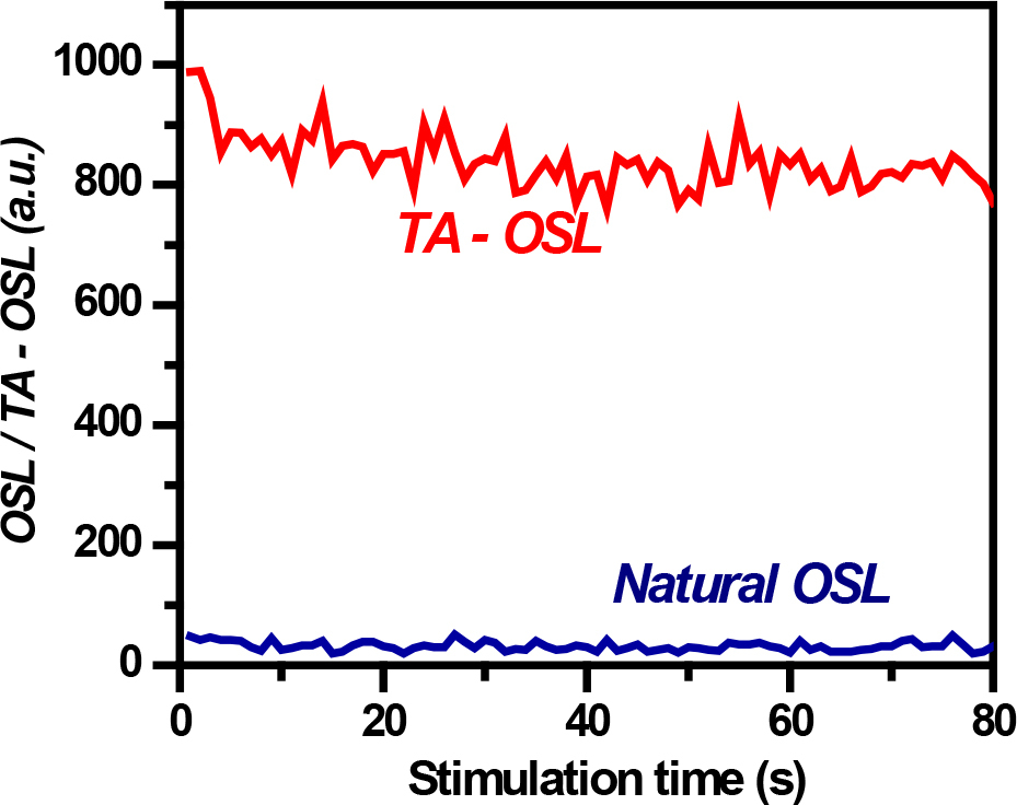
Fig. 1 presents typical OSL as well as thermally assisted optically stimulated luminescence (TA – OSL, Polymeris, 2016) signals from one CaCO3 sample of the present study following natural irradiation, namely without any artificial irradiation in the laboratory. The OSL signal was measured at 110°C, while the TA – OSL at 200°C. It is obvious from this figure that both signals consist of one component with shape rather peculiar and extremely flat. In terms of intensity levels, while the OSL indicates a signal similar to background, the TA – OSL yields intensity as large as ∼18 times the OSL background signal. As this figure reveals, a fast decaying component is missing from both signals. Neither the intensity nor the shapes of both OSL signals do change, even after illumination up to 1 ks using blue LEDs. This result indicates that these signals are extremely hard to bleach, at least within relative short time intervals. These features stand as indirect indications regarding the lack of significant quantities of either quartz or feldspar inclusions inside the clear CaCO3 precipitate. The lack of both quartz and feldspar inclusions could be further supported by the contents of Si and Na/K respectively, according to Table 1. In agreement with the previous reports by both Liritzis (1989; 2000; 2011) and Galloway (2002) we conclude that both OSL signals are not useful for luminescence dating. This is the reason why, for dating applications, the luminescence applications to calcium carbonates so far were limited to TL of mostly biogenic calcite (Duller et al., 2009; Liritzis, 2010; 2011; Polymeris et al., 2016). The TL signal of CaCO3 samples is known to be bleachable, however, prolonged bleaching times are required (hours or even days, McDougal, 1968; Liritzis, 1989; 2000). For a recent, indicative example, the authors could refer to Fig. 6 of Polymeris et al. (2016).
ED determination using the plateau method
The natural TL glow curves of all samples exhibit the same main characteristics, namely a glow curve that has the form of a continuum with two distinct but overlapping TL peaks at 325 and at 450°C (Fig. 2a). Figs. 2b and 2c present the MAAD TL analysis results for the sample SB1, which are representative for all the samples that were subject to the present study.
Fig. 2
Typical results of the MAAD plateau method applied for sample SB1. Plot (a) presents a NTL glow curve (as an average of three independently measured glow curves), plot (b) presents the representative Si curves for a selection of additive doses according to equation (2) while plot (c) presents an ED plateau versus glow curve temperature according to equation (1). Error bars correspond to 1σ.
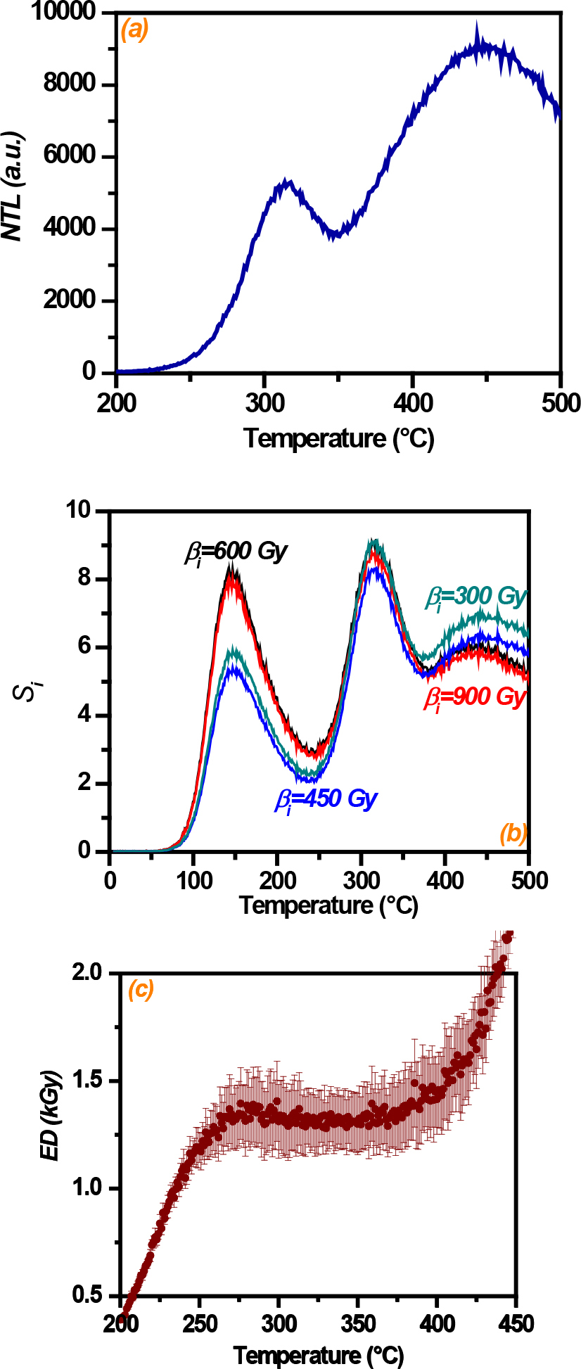
Fig. 2b presents the curves corresponding to the dose–response slopes (Si) which are plotted versus temperature for a selection of different additive doses applied for the sample SB1. Si curves were calculated according to Eq. 2.2 and the preceding subtraction takes place for each data point of the glow curves. According to Fig. 2b, these Si curves coincide, throughout a wide temperature region of the glow curve, namely between 250 and 400°C, confirming thus the dose response linearity within this aforementioned temperature range, despite the large additive doses. Consequently, the ED plateau is expected within the temperature range between 250°C and 400°C. Similar linearity Si features were also indicated for the rest of the samples.
Equivalent doses were calculated using Eq. 2.1. Since (a) all TL curves were measured using 500 data points and heating rate of 1°C/s up to a maximum temperature of 500°C and (b) the calculations take place for each data point of the glow curves, an ED value correspond to each TL glow curve temperature. If one plots these ED values versus the TL temperature, an ED plateau is expected to occur. A typical plot of ED plateau against glow curve temperature is presented in Fig. 2c. Errors, which are derived mainly from the uncertainties in curve fitting, are ±1σ and were calculated by standard error propagation analysis. In all cases, ED plateaus are wide enough, over 100°C wide. The equivalent doses were obtained as the mean values of the plateaus for each sample. Quite large ED values were obtained, ranging between 781(±71) and 1458(±166) Gy. Only linear fittings were performed to the dose response curves. Details of this ED calculation, such as the length, the value and the error of each ED plateau are presented for all samples in Table 2. It is worth emphasizing that for the estimation of the ED plateau region, all reheats (background TL glow curves) were subtracted. Moreover, for all samples the temperature range corresponding to the ED plateau lies within the temperature range of linearity according to the Si curves. Low dose supralinearity was not observed.
Table 2
Data related to the ED estimation for all four samples.
Deconvolution results and component resolved ED estimation
Fig. 3 presents a NTL + β (450 Gy) glow curve, deconvolved into its individual TL peaks according to Eqs. 2.3–2.5. For all NTL + βi glow curves, six individual TL glow peaks were used in order to achieve fit of excellent quality (FOM <0.9%). Nevertheless, for the case of the NTL glow curves, only three TL glow peaks are required (namely P4, P5 and P6) in order to achieve fit of ex cellent quality. A TL background curve has also been included within the deconvolution procedure, as Fig. 3 indicates. Table 3 presents an outline of the deconvolution analysis results, including the values of Tmax, activation energy E and the parameter R which gives information on the order of kinetics. It should be emphasized that the results obtained for all four samples studied were similar. The reproducibility of the Tmax values with ranging additive doses stands in excellent agreement with the R values of <0.1. Moreover, based on the deconvolution results, the lifetimes of the TL traps included in the NTL glow curves are adequate enough for providing ages of the order of 1 Ma.
Fig. 3
Representative deconvolution analysis of a TL glow curve corresponding to the sample SB1, after a dose of 450 Gy (open data points). Six different TL glow peaks and a black body radiation curve (BGK) were used in order to fit the experimental glow curve. Each TL glow peak is presented in solid line and is denoted as Pi. Orange solid line indicates the fitting curve. Table 2 indicates the activation energies of the TL peaks.
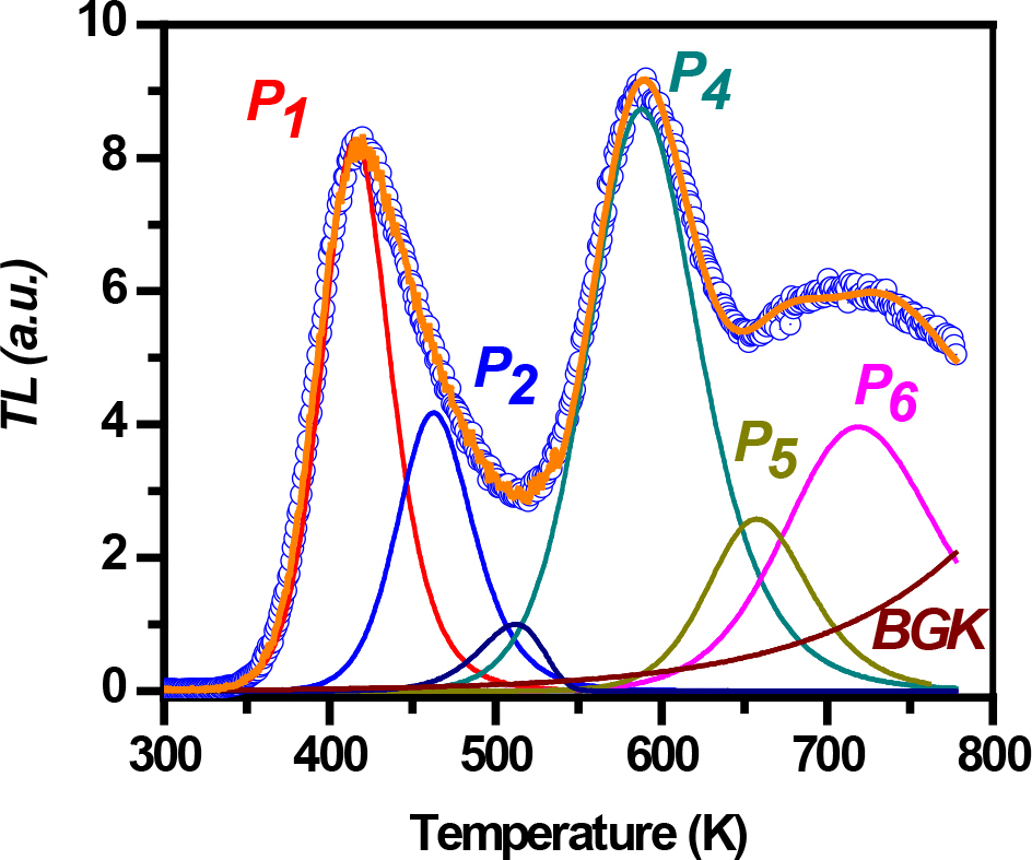
Table 3
Deconvolution results for fitting parameters of all four samples.
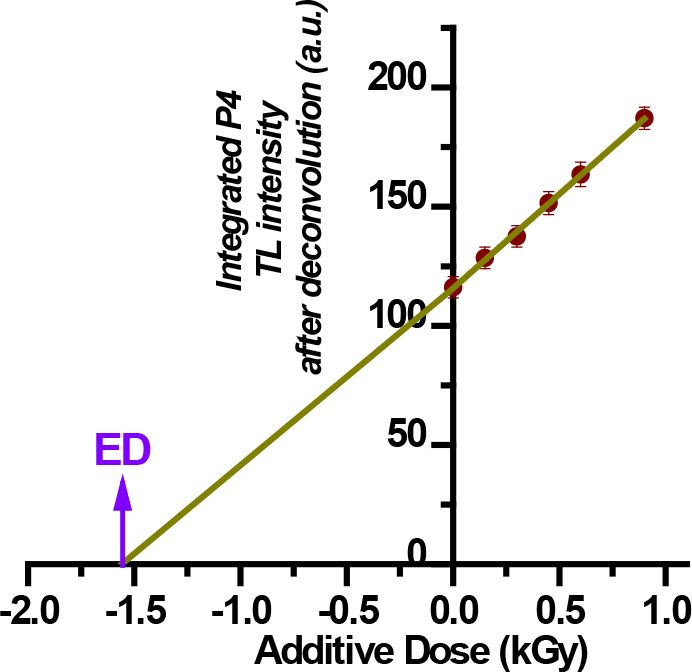
Besides the ED plateau method, equivalent doses were also calculated using the integrated TL intensity of each one of the three TL glow peaks which were used to deconvolve the NTL glow curves. An outline of the TL peak resolved ED estimation results could be found in Table 2. TL glow peak P4 is quite prominent, indicating very intense signal. The fitting parameters corresponding to this specific TL peak yield the lowest error values. However, the equivalent dose values calculated using the deconvolved integrated specific TL peak are overestimated when compared to the ED plateau value. Fig. 4 presents a representative additive dose response curve corresponding to sample SB1, plotted for the case of the integrated intensity of TL glow peak P4 after deconvolution. Despite the fact that the additive doses extend up to 900 Gy, linearity of the TL signal is characteristic for all samples. ED is overestimated at 1578(±177) Gy, while the corresponding plateau ED was calculated as 1258(±155) Gy. Similar overestimation was also yielded while using solely the integral of P6 TL peak. Component resolved overestimation ranges between 8 and 26%, depending on the TL peak used. Nevertheless, the most prominent TL glow peak P4 yields the higher overestimation percentage (15–26%). This experimental overestimation could be attributed to the fact that temperature range of TL glow peak P4 does not coincide with the plateau region for all samples. The overestimation yielded using TL glow peak P6, ranging between 8–14%, could be attributed to the fact that the TL glow curve should be measured up to temperatures higher than 500°C. As this is not the case, the resolution of the deconvolution technique is not the optimum. On the contrary, the additive dose procedure using the TL glow peak P5 yields the most comparable ED results with the ED plateau methodology. This similarity is quite prominent from the results of Table 1 and it is attributed to the fact that TL peak P5 lies within the corresponding plateau temperature range. Once again, it is worth noting that for all four samples and all three TL peaks, the linearity is quite impressive, despite the high additive doses applied.
TL ages
Estimation of the uranium, thorium and potassium geochemical content of the samples in the present study is currently pending. According to previous related luminescence studies using CaCO3, this geochemical content is quite low, indicating annual dose rate values lower than 1Gy/ka (for example Liritzis, 2010; 2011; Polymeris et al., 2016). Based on this rationale, the TL ages of these samples could reach values at least of 1 Ma, or even higher, namely in the Quaternary era. Nevertheless, as the present manuscript aims at presenting methodological aspects, as it was the case of the report by Duller et al., (2009), the detailed presentation of an integrated study dealing with the ages and their geological implications will be presented elsewhere.
. CONCLUSIONS
- The present study provides methodological aspects on the ED estimation for travertine samples, namely calcium carbonate samples, using the multiple-aliquot additive-dose procedure in TL.
- Heated CaCO3 can be effectively used for calculating equivalent doses within the range 750–1300 Gy.
- OSL and TA – OSL curves were measured and proven inappropriate for age assessment.
- The integrated intensity of TL glow peak P4 after deconvolution, provides age overestimation, compared to the age provided using the plateau method. This overestimation could be attributed to the fact that temperature range of P4 does not coincide with the plateau region of each sample.
- Using the integrated intensity of TL glow peak P6 after deconvolution is not suggested, as the resolution for resolving this peak is not good. As a result of this poor resolution, ED overestimation is also monitored.
- The integrated intensity of TL glow peak P5 after deconvolution provides ED values compatible with those yielded using the plateau methodology within the entire TL glow curve, with better accuracy, namely lower error values.
- The present study suggests not using the TL intensity (neither in terms of integrated intensity nor of peak height intensity) for ED estimation; instead it is highly recommended to use either the plateau methodology, or alternatively integrated intensity of TL peak P5 after deconvolution. Unfortunately, using the peak height of TL P5 is not recommended, due to overlapping with P6.
- TL age results indicate a formation during the Quaternary.