
. Introduction
Assessment of volcanic hazards relies upon characterisation of the nature and frequency of eruptions in a given area. While the first of these is typically accomplished via geochemical analyses, frequency modelling requires accurate and precise eruption ages. Despite many advances in the past 20 years, there are still a number of impediments hindering the dating of eruptions, particularly of Holocene basaltic rocks. Argon–argon dating, in which the amount of 40Ar produced by post-cooling radioactive decay of 40K is used to calculate an age, is the most common method for directly dating eruptions. In order to precisely date eruptions younger than ca. 100,000 years old, K-feldspar crystals must be present; only these reliably yield concentrations of potassium high enough to provide measurable amounts of argon (Mark et al., 2014). For understanding modern-day volcanic risk, it is precisely these young eruptions that must be dated, yet many of the most explosive eruptions do not provide the necessary minerals. Other decay-based dating methods, such as uranium–thorium and radiocarbon dating, may also have significant issues. Radiocarbon dating relies on the presence of appropriate organic samples of less than ca. 50,000 years in age, which may be rare in areas prone to extensive volcanic eruptions, while uranium–thorium dates require precise estimations of the initial isotopic ratios. Finally, cosmogenic nuclide (in particular 3H) surface exposure dating may be applied to lava flows (Craig and Poreda, 1986; Laughlin et al., 1994; Espanon et al., 2014b), but this technique has relatively low precision, requires extensive sample preparation, and assumes that the surface has not been substantial altered after deposition. It also cannot be used to date basaltic tephra or buried volcanic rocks.
Luminescence dating may be a suitable geochronological technique in these problematic settings. The method relies upon calculation of an absorbed environmental dose (‘equivalent dose’ or De) via the stimulation and emission of photons (‘luminescence signal’) from mineral crystals. The luminescence signal increases with time after the crystallisation and cooling of minerals — as in the case of volcanic phenocrysts — and can be reset by exposure to light or heat during transport — as for volcanic xenoliths or baked sediments. After estimation of the average environmental dose rate to the sample (Ḋ), time elapsed since the last resetting event or crystallisation can be calculated as: Age = De/Ḋ.
While luminescence methods have been used to date silicic volcanic rocks (see review by Fattahi and Stokes, 2003; Bösken and Schmidt, 2020), nearly all previous applications have relied on either quartz or K-feldspar. The plutonic varieties of these minerals have been thoroughly characterised by hundreds of luminescence studies (cf. reviews by Wintle, 2008; Preusser et al., 2009), but volcanogenic crystals manifest significantly different characteristics. Luminescence emission intensity, wavelength and response to radiation dose may vary, with the key difference being the seemingly universal presence of anomalous fading (Wintle, 1973). This process, in which the luminescence signal decays during storage, is distinct from the expected loss of thermally unstable charge, and most probably results from electron tunnelling (Visocekas, 2002). Without correction, anomalous fading will result in an underestimation of the luminescence ages. Although plutonic feldspar crystals commonly suffer from anomalous fading (Huntley and Lamothe, 2001; Auclair et al., 2003), experiments on volcanic feldspars have demonstrated extremely high signal loss rates (Gliganic et al., 2012). Unexpectedly, volcanogenic quartz also suffers from significant anomalous fading (Bonde et al., 2001; Tsukamoto et al., 2007), while anomalous fading has not been demonstrated for plutonic quartz. Such high fading rates, which are attributed to disorder in the crystal structure (Visocekas et al., 1998), invalidate some of the assumptions used in typical age correction models (Huntley and Lamothe, 2001). Therefore ‘corrected’ ages may still underestimate (by more than half) the expected ages based on independent age control (Tsukamoto et al., 2007; Thiel et al., 2015). While the effects of anomalous fading can be potentially reduced or avoided by either using red emissions (Hashimoto et al., 1986; Pilleyre et al., 1992; Fattahi and Stokes, 2000) or elevated temperature measurements of the optical signal (Tsukamoto et al., 2010; Tsukamoto et al., 2013), these techniques are still under development and may not be applicable to all volcanic environments (e.g. Richter et al., 2015). As both quartz and feldspar minerals may be problematic in volcanic settings, and in order to expand luminescence dating to intermediate and mafic volcanic rocks, characterisation of new luminescence dosimeters is desirable.
Olivine is the most common rock-forming silicate mineral on Earth, and it is the principal component of the Earth's upper mantle. It is omnipresent in most mafic and ultramafic intrusive rocks, such as gabbro and peridotite, but it also occurs in certain metamorphic rocks and extrusive rocks such as basalt. Olivine has also been detected in numerous meteorites and seems to be a major component of extra-terrestrial, rocky moons and planets in our solar system and beyond (de Vries et al., 2012; Sivakumar et al., 2017; Rubin and Ma, 2017). It has therefore been suggested as a potential target mineral for dating Martian deposits (Lepper and McKeever, 2000; Jain et al., 2006; Tsukamoto and Duller, 2008). To date, only a handful of publications have attempted to use or characterise mafic minerals for luminescence dating (Jain et al., 2006; Takada et al., 2006; Tsukamoto and Duller, 2008; Tsukamoto et al., 2011), and ever fewer publications have characterised pure olivine (Jain et al., 2006; Takada et al., 2006; Colin-Garcia et al., 2013). Importantly, the preliminary evidence available suggests that the luminescence characteristics of mafic minerals may be strongly variable based on the particular geochemistry of the volcanic deposit (Takada et al., 2006; Colin-Garcia et al., 2013).
This paper provides a systematic screening of olivine samples from different origins as a propaedeutic set for potential future dating applications. Six petrographically and geochemically characterised olivine samples from four intraplate settings are studied: two mantle xenoliths (Lanzarote, Canary Islands), three samples of olivine phenocrysts derived from basalts (Eifel, Germany; Lanzarote, Canary Islands; Argentina) and loose olivine grains from a sand beach (Hawaii). Thermoluminescence (TL) and photostimulated luminescence (PSL) properties are investigated, including emission wavelengths and intensities, growth of signal with absorbed dose, signal stability and recovery of a given dose with a PSL single aliquot regeneration (SAR) protocol.
. Structure and properties of olivine
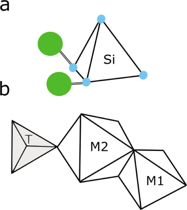
Olivine is a member of the orthosilicate class of minerals, which is defined by the basic chemical formula, Z:O = 1:4. For olivine, Z = Si, therefore the primary structure is defined by a silicon tetrahedron (SiO4; Fig. 1a). These isolated tetrahedral structures are joined laterally by Mg or Fe cations in octahedral coordination (Fig. 1; Bragg and Brown, 1926). The octahedral sites are not all identical, distorting the ideal hexagonal crystal structure and resulting in an orthorhombic structure (Bush et al., 1970). These distortions (M1 and M2, Fig. 1b) are occupied mainly by Mg and Fe, creating the two primary varieties of olivine, forsterite (Mg2SiO4) and fayalite (Fe2SiO4); other types, such as tephroite (Mn2SiO4), are rare. Generally, the olivine composition is defined in terms of the solid solution of the two end members, forsterite and fayalite: Fo80, for example, indicates that the composition of olivine is 80% forsterite and 20% fayalite. Forsterite is the first olivine type to crystallise from the melt as the temperature decreases to 1,890°C at one atmosphere pressure; therefore, the most primitive olivines will have the highest forsterite and the most magnesium (highest Mg#). Depending on chemical composition, the density of olivine is between 2.5 g·cm−3 and 2.9 g·cm−3.
Fig 1
Olivine structure. A) Silicon tetrahedra (blue spheres are oxygen) are laterally joined by Fe or Mg (large green spheres) to the next tetrahedral. Modified from Nesse (2012). B) M1 and M2 are octahedral sites. Note that site M1 is more distorted than M2. T indicates the centre of the tetrahedron.
Olivine is a readily available mineral among mafic rocks (dark volcanic rock with high concentration of ferromagnesian minerals) in various tectonic settings (midocean ridge, intraplate, subduction-related). The process of mineral nucleation from a melt is complex, as the system not only requires the appropriate chemical components to be present, but also the new mineral free energy of formation has to be lower than the same elements as part of the melt (Nesse, 2012). In addition, the amount of nucleation is related to the cooling temperature. In this sense, fast cooling lavas such as in volcanic rocks have high activation energy, hence, a high amount of small nucleation. This results in many crystals growing simultaneously, therefore limiting the size of each crystal. The growth rate of a crystal is determined by the surface energy, which is also tightly associated with the cooling rate. Therefore, the lower the surface energy, the larger the crystal. Furthermore, as the crystal grows, the crystalline structure of the mineral will develop point, line or planar defects (Nesse, 2012). These defects are very important for luminescence as they constitute the traps in which electrons will be held. It is important to note that basalts generally erupt at 1,100°C to 1,250°C, therefore constituent olivines have already crystallised.
. Sample setting and description
Samples were collected at five locations from similar, mainly intraplate tectonic settings (Table 1). Two samples were collected from Lanzarote, Canary Islands (Spain). Sample LZ2 is a peridotite xenolith from Pico Partido volcano and belongs to the AD 1730–1736 Timanfaya eruption (Aparicio et al., 2006). Sample LZ4 corresponds to the AD 1824 eruption of the Tinguatón volcano (Carracedo et al., 1992). This particular sample contains two types of olivine phenocrysts: (1) the ones that crystallized out of the magma and (2) the ones that were carried with the magma from the upper mantle and are part of a xenolith, which has crystallized long before transportation. In the case of sample LZ4 the xenolith mainly comprises olivine (>50%), hence it is called peridotite xenolith, and the size of the olivine phenocryst is >500 μm, while the material engulfing the xenolith is basaltic in composition and contains smaller olivine phenorysts. Therefore, two olivine subsamples were analysed from this rock, one from the basaltic groundmass (LZ4-B) and one from the xenolith (LZ4-X). Sample E-1 was collected close to the town of Sankt Johann in the East Eifel Volcanic Field (Germany). The age of the eruption is expected to be between 410 ka and 470 ka, as it is part of the Rieden volcanic complex (Bogaard et al., 1987). Sample HB is composed of sand-sized olivine grains from the Pu`u Mahana Beach, Hawaii (USA), where grains accumulate as the adjacent cinder cone erodes. According to Walker (1992), the eruption that produced this cinder cone exceeds 28 ka in age. Repeated bleaching and dosing of sedimentary grains in this sample may have altered their luminescence properties, as observed for quartz that has undergone several sedimentary cycles (Pietsch et al., 2008). Sample VRE-42 from the Llancanelo Volcanic Field (Argentina) was collected 450 km from the closest plate boundary and corresponds to back-arc extension volcanism, as the subducting slab has hinged back and created a gap for mantle upwelling. Geochemically, this sample has a weak subduction-related signature (Espanon et al., 2014a). All samples selected for this investigation yielded fresh olivine grains, which do not show alteration.
Table 1
Olivine sample details.
. Methods
. Mineral Separation
Rock samples were crushed using a press bench to obtain fragments <2 cm in size, after which their grain size was further reduced using a jaw crusher. Subsequently, samples were washed with distilled water, dried and sieved to obtain 200–400 μm grains. An olivine-rich fraction was extracted by magnetic separation with a hand-held magnet, followed by density separation using diiodomethane (ρ < 3.3 g/cm3). Non-rock sample HB contained shell fragments and was first washed in 5% HCl for 20 min, then rinsed with distilled water. The grain size of this sample was reduced using a mortar and pestle and sieved to obtain 200–400 μm grains. In order to assure the purity of the tested mineral fraction, olivines from all samples were hand-picked under a binocular microscope. During this step, composite olivines (olivines with groundmass attached), altered olivines and any other minerals were removed.
. Petrographic and Geochemical Analysis
Thin sections (one per sample, excluding loose HB grains) were prepared and analysed at the University of Freiburg. Previously cut, fresh rock surfaces were mounted on a glass slide with Körapox 439 resin, after which the remaining bulk was removed. Slices were first reduced to ~80 μm thickness via a ball mill, then the final thickness (~30 μm) was acquired by hand grinding using SiC 600–100 grit. The thin sections were polished using a Logitech WG2 polishing machine with MetaDi Supreme Polycrystalline Diamond Suspension with 9 μm, 3 μm and 1 μm abrasive particles, after which the sections were cleaned in an ultrasonic bath and with ethanol. All thin sections were observed under a Leica petrographic binocular microscope.
Two geochemical characterisation methods were used. Electron Micro Probe (EMP) analysis was performed for the five rock samples, using a Cameca SX100 EMP with an acceleration voltage of 15 kV, 20 nA maximum probe current and a raster length of 30 μm. The acquisition time was 40 s for K, 30 s for Cr and 20 s for all other elements. The San Carlos olivine standard (Jarosewich et al., 1980) was used for calibration. A minimum of four individual, similarly sized olivines were analysed per sample. Unconsolidated sample HB was analysed by Laser Ablation — Inductively Coupled Plasma — Mass Spectrometry (LA-ICP-MS), at the Institute of Geological Sciences, University of Bern. Olivine grains were crushed and pelletised, after which the olivine pellet was analysed by a GeoLas-Pro 193 nm ArF Excimer laser system (Lambda Physik, Germany) in combination with an ELAN DRC-e quadrupole mass spectrometer (Perkin Elmer, USA). Measurement standards SRM612 and GSD-1G were used. Six measurements were recorded, which have been averaged for the final reported value.
. Luminescence Characterisation
Stainless steel cups (provided by Freiberg Instruments), tweezers and work surfaces were carefully cleaned immediately prior to aliquot preparation. Preparation took place in a low-dust environment not typically used for luminescence sample preparation (no red-light illumination). Aliquots were prepared by loading loose olivine grains into stainless steel cups until the entire surface of the cup was covered by a monolayer of grains. These were immediately covered with foil after preparation in order to prevent any contamination, and then the cups were transferred into the cleaned carousel of the luminescence reader.
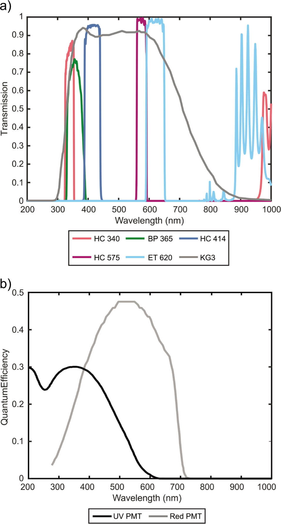
An automated Lexsyg Research TL-OSL system (Richter et al., 2013) was used to characterise the luminescence properties of the olivine grains. Samples were stored within a light tight, 80-position carousel, and transferred to the measurement chamber and measured one-by-one. Beta irradiation of samples was conducted with a planar 90Sr/90Y RFQ-2 source providing c. 0.12 Gy·s−1 to coarse grains on stainless steel. A ceramic heater plate was used for linear ramping to a maximum temperature of 500°C and stable heating of the aliquot cups during TL and PSL measurements. Optical stimulation was provided by one interchangeable PSL unit comprising 15 LEDs in three emission wavelengths: blue (LZ1-00B200: 458 ± 5 nm, 100 mW·cm−2), infrared (IR) (LZ1-00R400: 850 ± 20 nm, 300 mW·cm−2) and yellow (LZ1-00A100: 590 ± 30 nm, 20 mW·cm−2). A fused quartz biconvex collecting lens located in the PSL unit increased light collection efficiency. Two six-slot filter wheels allowed a number of different filter combinations to be easily tested during these experiments. Filter details are provided in Table 2, and transmission characteristics for each filter are shown in Fig. 2a. In the remainder of the paper, the filter combinations will be referred to by the wavelength of their nominal peak transmission (i.e. 330, 380, 410, 565 and 620). These transmissions may also be referred to as UV (330 and 380 nm), blue (410 nm), yellow (565 nm) and red (620 nm). Luminescence signals were detected by two photomultiplier tubes (PMT), an extended UV/blue optimised (Hamamatsu 9235QB) unit and a red-enhanced UV-Visible GaAsP photomultiplier (Hamamatsu H7421-40 ‘Photon Counting Head’). The quantum efficiency (QE) curve for each PMT is shown in Fig. 2b.
Table 2
Filter and PMT details. a) Detection packs (filters + PMT) for TL emission measurement. All detection packs use a Schott KG3 (3 mm) as one of two filters; the second filter slot is variable. Transmitted flux refers to the integrated flux through each filter set as a proportion of the total possible transmission, and the calculation for N is given in the text. b) PSL filter combinations used, always detected with UV PMT. No normalization is applied.
Fig 2
Filter and detection equipment characteristics. A) Transmission curves for all filters and B) quantum efficiencies of the Hamamatsu 9235QB (‘UV PMT’) and Hamamatsu H7421-40 Photon Counting Head (‘Red PMT’). PMT, photomultiplier tubes.
Multiple TL and PSL experiments have been undertaken in order to characterise luminescence emissions from the olivine grains. Measurement protocols are described below and in Figs. 3 and 4. Calculation of Lx/Tx values has been carried out via Risø Luminescence Analyst (Duller, 2013). All other analyses are described in detail below, and they have been carried out via MATLAB scripts written by one of the authors (LAC).
Fig 3
TL characterisation protocols: Protocols A and B. The flow chart defines the sequence of steps for a single aliquot, with white boxes indicating steps that only occur once and grey indicating repeated steps. The repeating portions of the method are indicated with an arrow and an integer indicating the number of repetitions. For each repetition, any changing experimental parameters are indicated in brackets (<>). For example, the steps in Protocol A are carried out seven times total, and each time a different filter pack is used for the TL detection. TL, thermoluminescence.
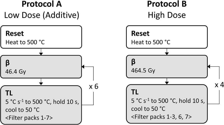
Fig 4
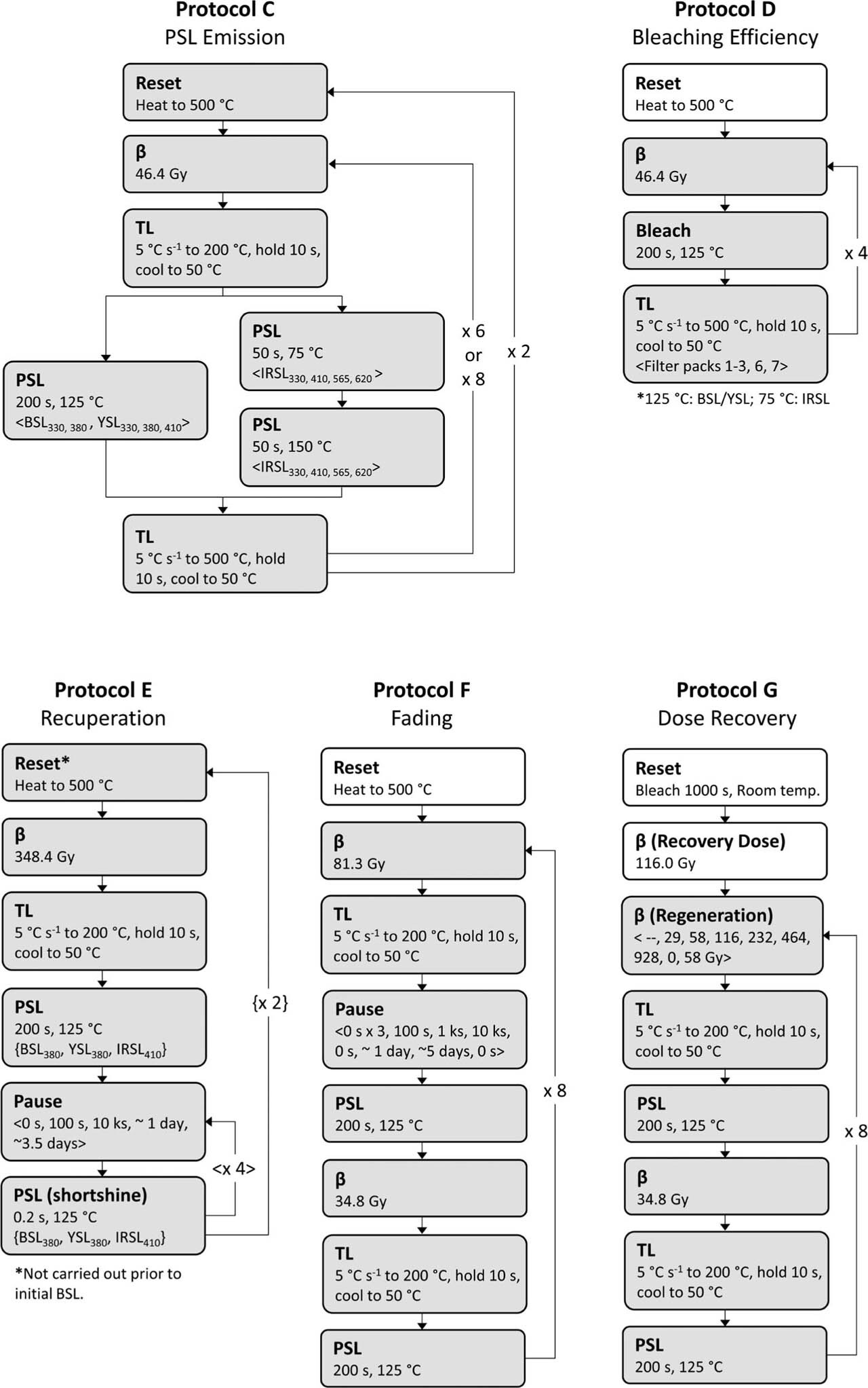
Photostimulated luminescence characterisation protocols: Protocols C–G. The flow chart defines the sequence of steps for a single aliquot (see Fig. 3 for more details). Protocol E involves two sets of repeated steps. The parameters that are changed in each set of repetitions are indicated by the enclosing punctuation, <> and {}.
. TL characterisation
TL emissions after irradiation with 46.4 Gy were characterised for three unmeasured aliquots from each sample according to Protocol A (Fig. 3). UV/blue emissions were detected with the UV-enhanced PMT, and both available PMTs were used to measure yellow and red emissions. After data processing, however, it became clear that the red-enhanced PMT provided a significantly higher signal-noise ratio for both yellow and red emissions. Therefore, for these emissions only the red-PMT results are reported in this study. Background values for each emission, which comprise thermally induced emissions from the disc and heating plate, were also measured for each aliquot via Protocol A with no irradiation step. Glow curves (post-irradiation and background) were interpolated onto the same temperature scale to correct for small inconsistencies in heating rate, after which the background data was subtracted from the post-irradiation data. This background corrected data was then normalised by the factor N described below.
Three aliquots were also given a higher beta dose to examine peak growth with laboratory dose (Protocol B, Fig. 3): one unmeasured aliquot each from samples HB and LZ4-X, and one of the previously dosed and TL measured aliquots from E-1.
The data from these experiments have been analysed as follows. In order to directly compare the magnitude of TL emissions detected via separate filter packs and with two different PMTs, it was necessary to apply a normalisation factor to each glow curve. This is a product of both the differing total intensity of light transmitted by the various filter packs and the different QE curves of the detection equipment. In general, the total amount of light detected by the PMT at a given time is the integral (over all wavelengths) of the product of the transmission curves of each filter and the QE of the detection equipment. Therefore, the true intensity of the emission can be estimated as:
where λ1,2 are chosen to encompass the effective QE of the PMT, T1,2 are the filter transmission curves and QE is the QE curve.Filter transmission characteristics and QE curves were provided by Freiberg Instruments. Curves for the KG3 filter and both PMTs were digitised from images provided by the manufacturers (Rohatgi, 2010). Filter sets used to detect emissions are listed in Table 2a. All transmission and QE curves (as a proportion of total intensity) were interpolated between 200 nm and 1000 nm (2 nm spacing) via Matlab ‘spline’. Negative values were then removed from the digitised data sets. For each wavelength, filter transmission values were multiplied with the QE curve of the appropriate PMT. Numerical integration was then performed over the range 200–1000 nm, to give the normalisation factor N (Table 2a).
. PSL Characterisation
After examination of the TL peak structure, a relatively low preheat temperature of 200°C (10 s) was selected for all PSL measurements (emission selection via filters given in Table 2b). PSL emission intensities (UV and UV/blue) were characterised for blue, yellow and IR stimulation for three unmeasured aliquots from each sample (Protocol C, Fig. 4). For this initial characterisation experiment, IRSL comprised two sequential measurements, the first at 75°C and the second at 150°C, to see how the crystals responded to a modified post-IR IRSL protocol (Thiel et al., 2011; Thomsen et al., 2008). The entire measurement cycle was repeated three times. IR/red detection (IRSL565 and IRSL620) was also tested with one of the above aliquots from each sample. Detectable emissions were defined by the presence of a signal (first 5 s) greater than three times the standard deviation above the background (last 10 s).
One previously measured aliquot from each sample (TL, Protocol A) was then measured via Protocol D (Fig. 4) in order to investigate differential bleaching efficiencies of blue, IR and yellow stimulation: after irradiation, a PSL step was inserted before TL measurement. TL measurements were made with all five filter combinations used in the TL characterisation above. LED intensity and heating for the bleaching step have been chosen to be the same as those used during the PSL characterisation and dose recovery protocols, therefore, the results presented are applicable to understanding what is occurring during the different PSL protocols.
Post-bleaching recuperation was tested via short-shine measurements (Protocol E, Fig. 4), in which a short stimulation pulse releases a negligible fraction of the trapped charge, ~1% (Smith et al., 1986). In this manner, ongoing signal buildup or decay can be monitored. One previously unmeasured aliquot from each sample was irradiated, bleached, then short-shine measurements were conducted after storage periods ranging from immediate measurement to 3.5 days. Each short-shine comprised 0.2 s stimulation followed by continuing PMT recording for 1.6 s. Recuperation values are calculated as the net short-shine signal (intensity minus the average non-stimulation detection signal – dark current – of the PMT in the following 1.6 s) expressed as a percentage of the signal counts in the first 0.2 s of the post-irradiation PSL bleach.
Storage experiments were used to investigate the stability of the detected PSL emissions, via a sensitivity-normalised method comprising repeated irradiation and preheating prior to varying storage times (Auclair et al., 2003). Storage times ranged from immediate measurement to 5 days. Two aliquots from samples HB, LZ4-X, E-1 and VRE-42 were measured. All aliquots excepting one new aliquot from VRE-42 had been previously measured, including heating to 500°C. Five immediate measurements were included in the protocol (three at the beginning, one in the middle and one at the end) in order to test the accuracy of the test dose sensitivity correction. Test dose normalisation is considered acceptable if the normalised intensities of repeated steps (‘recycling ratio’) are within 15% or two sigma of the first step. Signal integration times are the first 4 s for BSL and YSL measurements, and the first 10 s for IRSL, and the last 40 s is used for background calculation. G-values have been calculated where applicable according to Huntley and Lamothe (2001).
Dose recovery experiments were carried out for previously unmeasured aliquots prepared from samples HB, LZ4-B, LZ4-X and VRE-42. Due to the limited sample quantities, only one aliquot each was measured for each of three stimulation/detection combinations (BSL380, IRSL410, YSL380), excepting VRE-42, for which only two aliquots were prepared (BSL380, IRSL410). Each aliquot was first bleached with the chosen stimulation light for 1,000 s at room temperature, after which they were beta irradiated (116.0 Gy). A SAR measurement protocol was used, with recycled and zero-dose steps (Murray and Wintle, 2003, 2000). The recycling ratio is the result of dividing the second by the first recycling measurement. The zero-dose comprises a ‘Pause’ block in the LexStudio software, with the aliquot held at the stimulation head position for 200 s. Zero-dose ratios were calculated by dividing the Lx/Tx value of the zero-dose measurement by the Lx/Tx value of the applied (recovered) dose measurement. All parameters were held constant between experiments (Fig. 4), except for the wavelength and intensity of the stimulation light and sample temperature during measurement. After the end of the primary dose recovery protocol, each aliquot was stored for between four and five days, and then the recuperated PSL signal was measured again (no preheat), followed by a standard test dose. Signal has been integrated from the first 4 s (blue) or first 10 s (IR and yellow stimulation), respectively (unless otherwise noted). The background has been calculated from the last 40 s.
. Results
. Petrographic Description
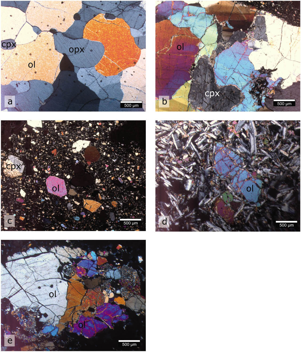
Olivine is the dominant mineral in the two xenoliths analysed. Due to the high olivine concentration (>40%), these two xenoliths are identified as peridotite xenoliths. In Fig. 5a and b other minerals can also be identified, such as orthopyroxene (opx) and clinopyroxene (cpx), but these only comprise a few percent of the xenoliths. Sample LZ2 has higher opx content than LZ4-X (xenolith), which in turn has a higher cpx content than LZ2. In sample LZ4-X, olivines are much more fractured than those found in sample LZ2, and slight alteration to the iddingsite can be observed along the fractures. The alteration of olivine to iddingsite is not abnormal, and it is also apparent in the olivine shown from sample VRE-42 (Fig. 5d). The basaltic components of sample LZ4-B (Fig. 5c) and sample E-1 (Fig. 5e) show a typical porphyritic texture. The phenocrysts from sample LZ4-B (Fig. 5c) are mainly olivine, opx and cpx, while the groundmass is composed of the same minerals as well as plagioclase. The sample from the Eifel Volcanic Field (E-1) is slightly different as it contains other minerals such as nepheline (Fig. 5e), which are typically found in alkaline rocks (rocks with high Na2O + K2O). The groundmass of this sample is composed of olivine, cpx, oxides and glass. The olivines from all samples are fresh despite the slight alteration to iddingsite observed in sample VRE-42. This sample (Fig. 5d) has an interstitial and intergranular texture. The phenocrysts are mainly olivine and cpx and majority of the groundmass is composed of plagioclase feldspars and some glass.
Fig 5
Analysed thin sections: A) LZ2, B) LZ4-X, C) LZ4-B, D) VRE-42, E) E-1. Photographs were taken using a binocular microscope (magnification ×4) under cross-polarised light. Examples of olivine (Ol), clinopyroxene (cpx) and orthopyroxene (opx) are identified in the images. Note that the black areas in (c) are vesicles.
. Major Element Composition
The values presented in Table 3 are average measurement values (samples VRE-42 and LZ4-B (n = 4); E-1 and HB (n = 6) and LZ2 and LZ4-X (n = 10)). The relative standard deviation is less than 5% for the most abundant major elements (SiO2, FeO, MnO and MgO); however, it is larger for the rest of the major elements as their concentrations are low in olivine and close to the instrumental detection limit.
Table 3
Major oxide composition of analysed olivines (in wt%).
Olivines from the two xenoliths have the highest MgO content as expected due to their primitive origins (Table 3). These olivines have been brought up to the surface within a short time period, therefore they retain a characteristic mantle composition. Since they did not have time to equilibrate with the basaltic melt in the magmatic chamber, xenolith olivines have a different composition than phenocrysts within the basaltic groundmass (Table 3). The lack of significant alteration and the primitive origin of the olivines are further evidenced by the high magnesium number (Mg#, Table 3). The olivines from the basaltic groundmass have higher FeO, MnO and CaO content and lower MgO and NiO than the olivines from the xenoliths. Sample E-1 has the most differentiated composition, according to the low Mg# and NiO content. Sample VRE-42 has a higher Fe content than other olivines in this study possibly due to some olivine alteration to iddingsite.
. TL Characterisation
Glow curves and interpolated (for heatmap visualization) TL peak structure from laboratory doses (46.4 Gy) are presented for a representative aliquot from each olivine sample (Fig. 6). Intra-sample variation was minimal, with central peak temperatures and relative magnitudes nearly identical. The largest variation occurred in the relative magnitude of the 380 nm peak for aliquots from samples LZ4-B. A UV/blue low temperature peak (90–100°C) seems to occur in nearly all samples. This comprises the dominant peak for samples LZ4-B and LZ4-X, but it also occurs at lower relative intensities for samples HB, VRE-42 and LZ2. Close examination suggests that this peak may also occur in the E-1 data, but if present, the emission is weak and difficult to distinguish from the rising edge of the 150°C peak. The central wavelength for this peak emission seems to be either 380 nm (common) or 330 nm (LZ2). The first half of another peak found in all samples is visible in the 410 nm glow curves at 400–500°C. This blue peak is dominant for HB, VRE-42 and LZ2. Further UV/blue emissions are apparent, but these tend to be indistinct ‘ramps’ rather than well-separated peaks (especially VRE-42 and LZ2). An exception to this pattern occurs with sample E-1, where overlapping but distinct, high magnitude peaks occur at 150°C and 290–300°C. A low intensity peak is also visible at 240°C.
Fig 6
Glow curve data is presented for low-dose TL characterization. Background subtracted and normalised glow curves are plotted over a heatmap and contour lines, indicating the temperature and wavelength of detected peaks. Heatmap and contours are intended for visualization; these have been estimated via interpolation of the measured glow curves and median filtering (window = 4 °C × 40 nm). Contours are drawn at intervals of 25,000 counts for samples E-1, LZ4-B and LZ4-X, and 10,000 counts for HB, VRE-42 and LZ2. Curve data has not been plotted at temperatures greater than 350 °C and 300 °C for yellow and red emissions, respectively, due to the high thermal background. Note also that luminescence count scales cover a larger range for E-1 and LZ4-X. TL, thermoluminescence.
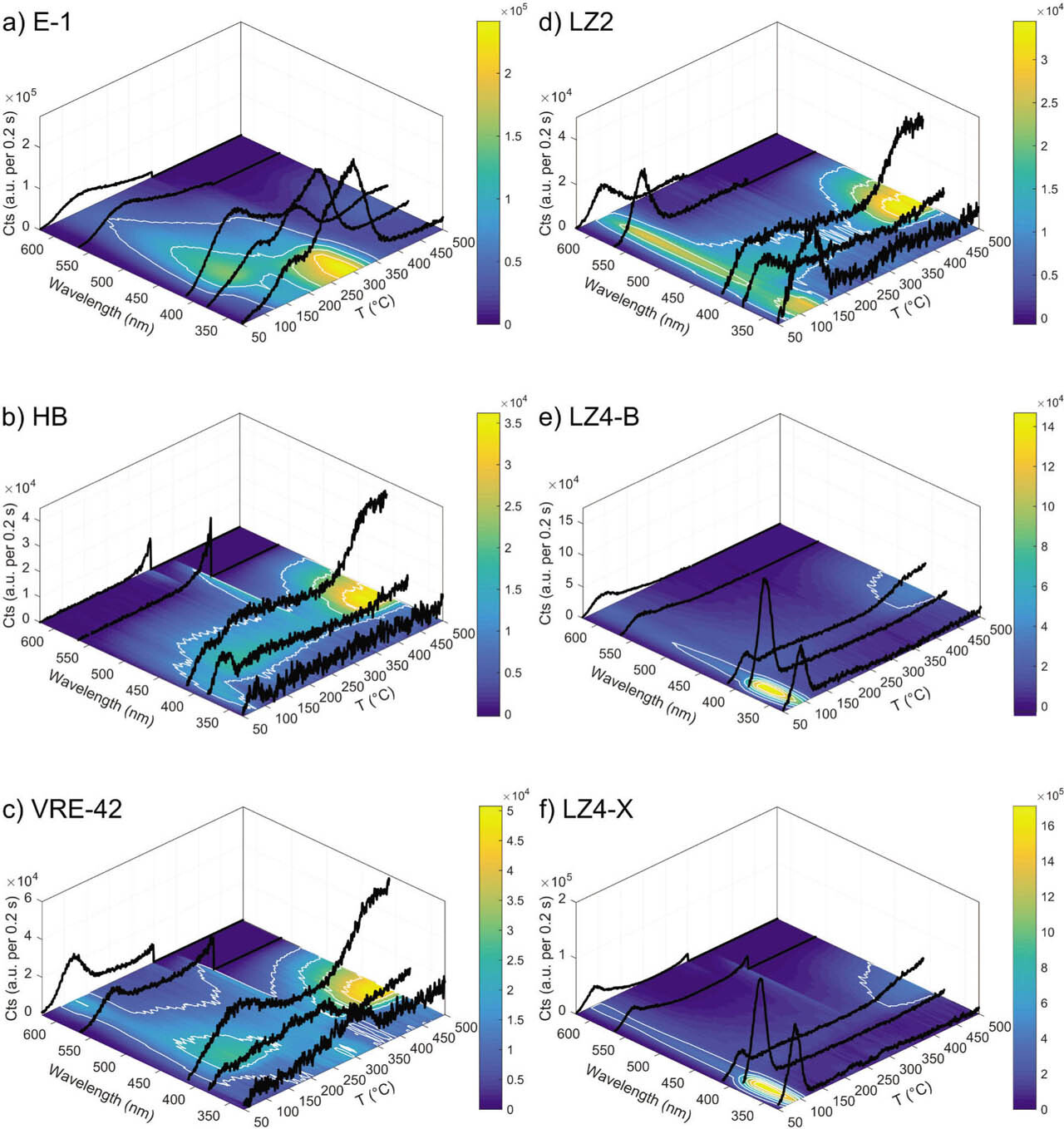
Red/yellow emissions are detected from all samples except for HB, and peaks tend to occur at similar temperatures and have similar relative intensities. Red emissions are of the same or higher intensities than measured yellow peaks for all samples except LZ2 and E-1. Single peaks are detected in red/yellow emission windows for E-1 (~150°C) and LZ2 (~100°C). Samples LZ4-B, LZ4-X and VRE-42 share a similar multiple peak structure, with a lower temperature primary peak and a higher temperature indistinct secondary peak. For LZ4-B and LZ4-X, the dominant peak occurs at 90–100°C with secondary, indistinct peaks at ~130–150°C, while VRE-42 peaks occur at ~125°C and 200–200°C.
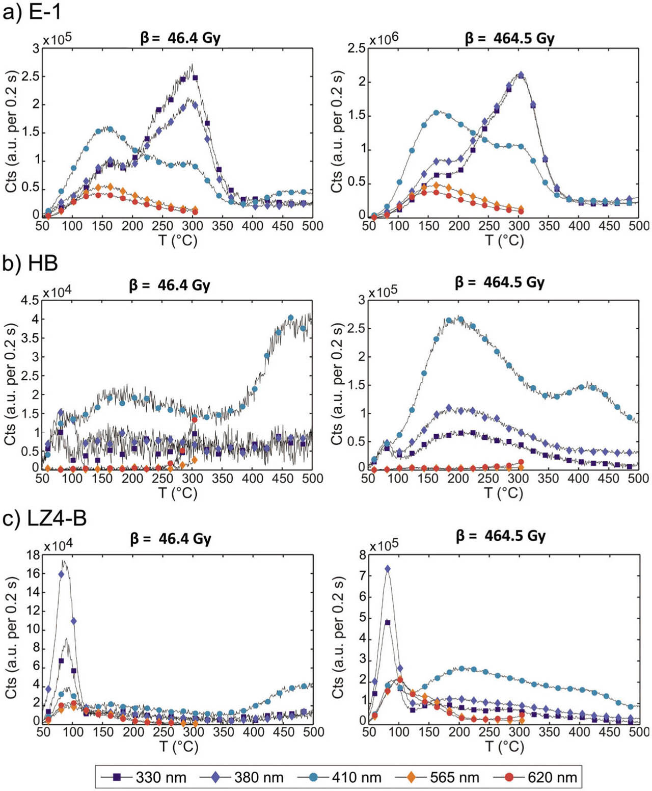
For the high-dose TL (Fig. 7), HB and LZ4-B olivines again share a similar peak structure. In the UV/blue region, the low temperature 90–100°C peak remains, but new peaks become visible at 200°C and 400–450°C. Both peaks are strongest in the 410 nm signal. A dim red/yellow peak (~4000 cts/0.2 s) at ~125°C is also induced in the HB olivine by the larger irradiation. For each sample, signal magnitude is increased by 3–4 times for the UV/blue low temperature peaks, and 10 times or more for the UV/blue higher temperature peaks and the red/yellow low-temperature peak. By contrast, the high dose irradiation of the previously measured E-1 aliquot yields enhancement of the previously apparent peaks between 6 and 10 times. No further peak structure becomes apparent. Measured peak structure in the Eifel olivines (Fig. 7a) still does not correspond with the peak structure of the HB and LZ4-B olivines (Fig. 7b, c), even at higher doses.
Fig 7
Background corrected low- and high-dose glow curves compared for samples A) E-1, B) HB and C) LZ4-B.
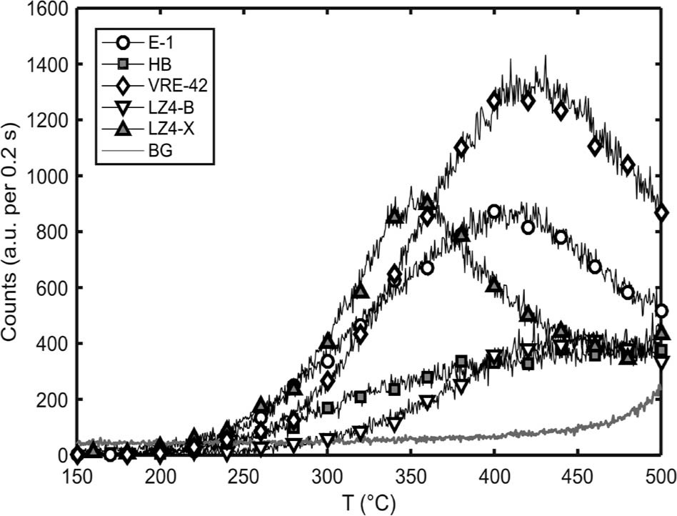
Remnant natural TL (410 nm) is apparent in measurements made prior to PSL characterisation in Protocol C for five of six samples (excluding LZ2; Fig. 8). All rock samples have been prepared in standard indoor office light conditions, and sample HB was collected from a beach surface fully exposed to daylight. Therefore, it appears that charge in traps >250–300°C is not or only very slowly bleachable.
. PSL Characterisation
All samples, every aliquot and every repeated measurement shared the same reliably detectable PSL emissions: all tested emissions for blue and yellow stimulation (BSL330, BSL380, YSL330, YSL380 and YSL410), and IR410 and pIR410. Three aliquots, one each from sample LZ4-X, VRE-42 and LZ2, also yielded just detectable IR565 emissions. All other IR/pIR stimulation steps yielded occasional signals just past the defined detection boundary; however, these never occurred reliably on each of the three repeated cycles. No measurements of IR620 emissions were possible, due to the high IR background (several tens of thousands of counts per 0.2 s).
Relative average intensities of the reliably detected PSL emissions are compared in Fig. 9a. These have been normalised by the total net PSL signal detected from each sample. Net signal intensities are in every case greatest for the 380 nm emission during blue and yellow stimulation, with the exception of sample LZ4-X, for which YSL410 was slightly brighter than YSL380. Sample E-1 yields the most unique signals, with a net BSL380 signal between 8× and 11× brighter than YSL380. In terms of absolute emission strength, E-1 olivines yield an initial BSL380 signal approximately three times brighter than all other olivine samples, which cluster around 1000 cts/0.2 s. Other emission intensities are dim but quite homogeneous between all samples. IR410 and YSL410 initial intensities are 273 ± 41 and 188 ± 54 cts/0.2 s, respectively (μ ± 1σ, all aliquots, all repeated cycles).
Fig 9
PSL properties of olivine samples. A) Net PSL signals as a proportion of the total net signal emitted by grains from each sample. Signal proportion and total signal are calculated for each sample from the average of all measured aliquots and each repeated cycle. Only reliably detected signals are included (see text). Decay curves from all measured aliquots are presented for B) BSL380, C) YSL380, and D) IRSL410 measurements (75 °C main plot, post-IR 150 °C inset). IR, infrared; PSL, photostimulated luminescence.
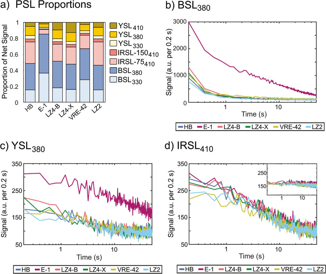
Representative decay curves for these signals (Protocol C) are plotted in Fig. 9b–d. Decay curves from bleached but unheated aliquots can be seen in Fig. 13 (Protocol G). All aliquots within a certain sample share the same basic decay curve characteristics, though these can vary between samples. For instance, BSL380 decay curves are the most variable, with Eifel olivines consistently showing a prominent decay component between c. 3 s and 20 s that is not apparent in grains from other samples. This pattern is also shown by VRE-42 olivines, to a much lesser extent. IRSL410 and YSL380 decay curves are much more homogeneous. Decay curve fitting was performed for BSL, IRSL and YSL emissions with single exponential and sums of up to four exponential decay functions. All curves are best fit by more than one exponential component, most often three. Variation in the dominance of each decay component can be seen in Fig. 9b, and particularly in Fig. 13. It is apparent that the BSL380 decay is most often dominated by the fastest decaying function, whereas IRSL410 and to a lesser extent YSL380 are dominated by a slower decaying component.
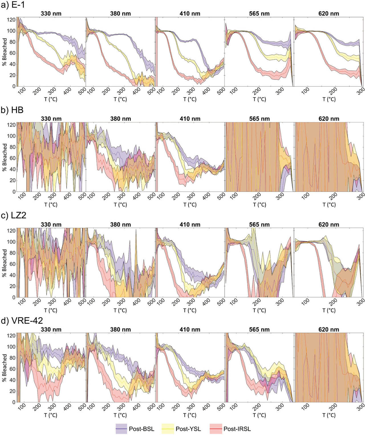
Inspection of the TL resetting steps in the above experiment revealed the existence of an incompletely bleached TL410 emission between 200°C and c. 325°C. The magnitude of this peak was similar after blue, yellow and IR bleaching for five of six samples. E-1, by contrast, showed a substantial and replicable decrease in remnant charge after BSL as opposed to YSL or IRSL steps. Protocol D was therefore conducted in order to investigate bleaching efficiency, by inserting a bleaching step between irradiation and TL measurements. Fig. 10 shows the results, with signal loss due to blue, yellow and IR stimulation plotted as a percentage of the unbleached glow curve intensity measured for the same filter combination during Protocol A. Unsurprisingly, the unstable low temperature peaks, below c. 100–125°C, are fully emptied by the PSL protocols used (stimulation plus heating). For olivines with detectable TL peaks between 150°C and 400°C (HB, VRE-42 and particularly E-1), charge is released by blue, yellow and IR stimulation in that order of efficiency. E-1 olivines appear to share a higher BSL bleaching efficiency (>80%) up to approximately 300–350°C, in contrast to the other samples; however, this is complicated by the dimness or absence of high-temperature peaks in the other samples. By approximately 400°C, yellow and IR stimulation seems to be as or more efficient at bleaching charge than blue light; however, this may be an artefact of the background subtraction.
Fig 10
Proportion of TL (%) bleached by blue, yellow or IR stimulation for samples A) E-1, B) HB, C) LZ2 and D) VRE-42. The bleaching percentage is sometimes greater than 100 due to analytical error. Subplots for each sample correspond to emission detection wavelengths, and line colours indicate the stimulation light. For example, it is apparent that for sample E-1 blue light bleaches nearly all TL signal in the 330 nm detection window for temperatures up to ~350 °C. IR, infrared; TL, thermoluminescence.
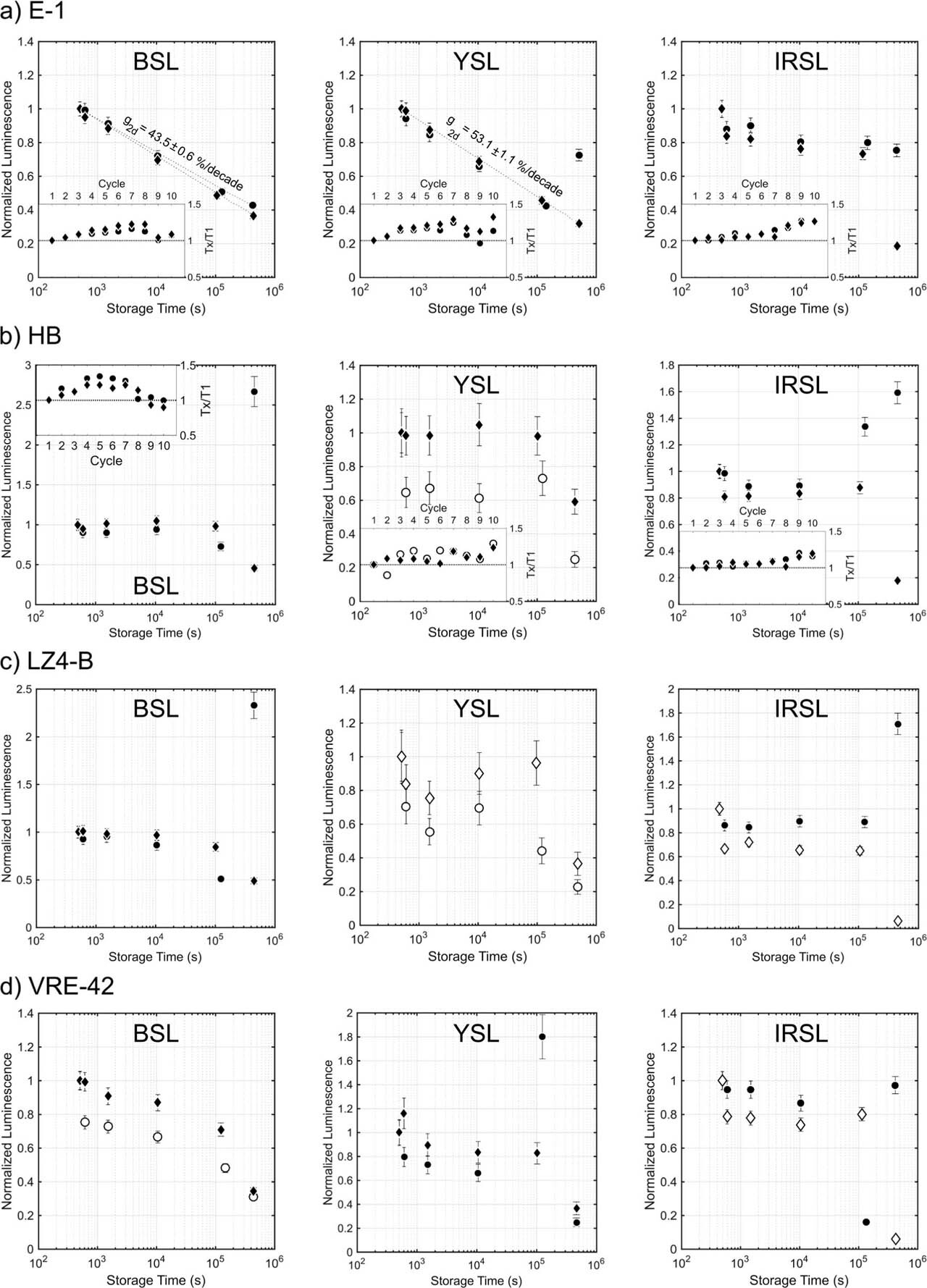
Fading experiment results are summarised in Fig. 11. Recycling ratios are unacceptable for one, two and three aliquots measured with BSL380, YSL380 and IRSL410 signals, respectively. Data for these aliquots are shown for completeness (indicated by white-filled symbols), but accurate measurements of signal instability in a regeneration protocol requires a stable, sensitivity-corrected signal. Accepted aliquots display complex relationships between signal magnitude and storage time. Only three sets of measurements, two E-1 aliquots measured via BSL380 and one E-1 aliquot measured via YSL380, show the expected linear decrease in signal with decade of time due to anomalous fading. For these aliquots, normalised signal intensity has decreased to less than half of its original value after 5 days of storage. g-values of 43.5 ± 0.6% per decade and 53.1 ± 1.1% per decade are calculated for BSL380 and YSL380 signals, respectively. By contrast, other aliquots show significant departures from expected linearity, with periods of signal stability, loss and even increase with storage time. These patterns do not correlate with Tx/T1 sensitivity change; therefore, this seems to be a true measurement of the signal behaviour through time. Signal increases do not seem to be due to incompletely corrected sensitivity changes, as can be seen by comparing the normalised luminescence changes and inset Tx/T1 values.
Fig 11
Results of storage experiments for samples A) E-1, B) HB, C) LZ4-B, D) VRE-42. For each sample, measured aliquots are distinguished by marker shape (circle and diamond). White-filled aliquots indicate that an aliquot failed at least one recycling ratio test. Test dose sensitivity change is shown in the inset boxes for E-1 and HB. Note that the sensitivity patterns do not correlate with ‘outlier’ intensity measurements. Calculated g-values (tc = two days) are also given (see text for details).
Both short-shine measurements (Fig. 12) and zero-dose ratios (immediate and five days, Table 4) have been examined for signal recuperation. A wide variety of behaviour is apparent; however, some patterns can be seen. Short-shine measurements indicate that BSL380 recuperation levels tend to be less than 5% of original PSL intensity, even after storage for several days. The exception to this is sample HB, which yields a significant (>20%) recuperation value by 1 day of storage. In contrast to this, YSL380 signal recuperation rises to ca. 20% by the first day for all aliquots, then remains stable or decreases by three days of storage. IRSL410 results are more mixed, with some high and some negligible recuperation values. Interestingly, five days zero-dose ratios tend to show a different pattern (Table 4), with BSL signal recuperation at a very high level. BSL380 measurements show that while HB signal recuperation is again the most significant (88.4% recuperation), both LZ4-X and VRE-42 recuperated 14–20% of their original signal. IRSL410 recuperation is again problematic for HB (36.6%); however, samples LZ4-B, LZ4-X and VRE-42 have zero-dose ratios less than 5%. Recuperation is similarly low for YSL380 measurements upon samples HB and LZ4-B.
Fig 12
Short-shine recuperation as a percentage of initial PSL intensity (Step 6, Protocol E) measured for all olivine samples: A) BSL380, B) YSL380, C) IRSL410 75 °C. PSL, photostimulated luminescence.
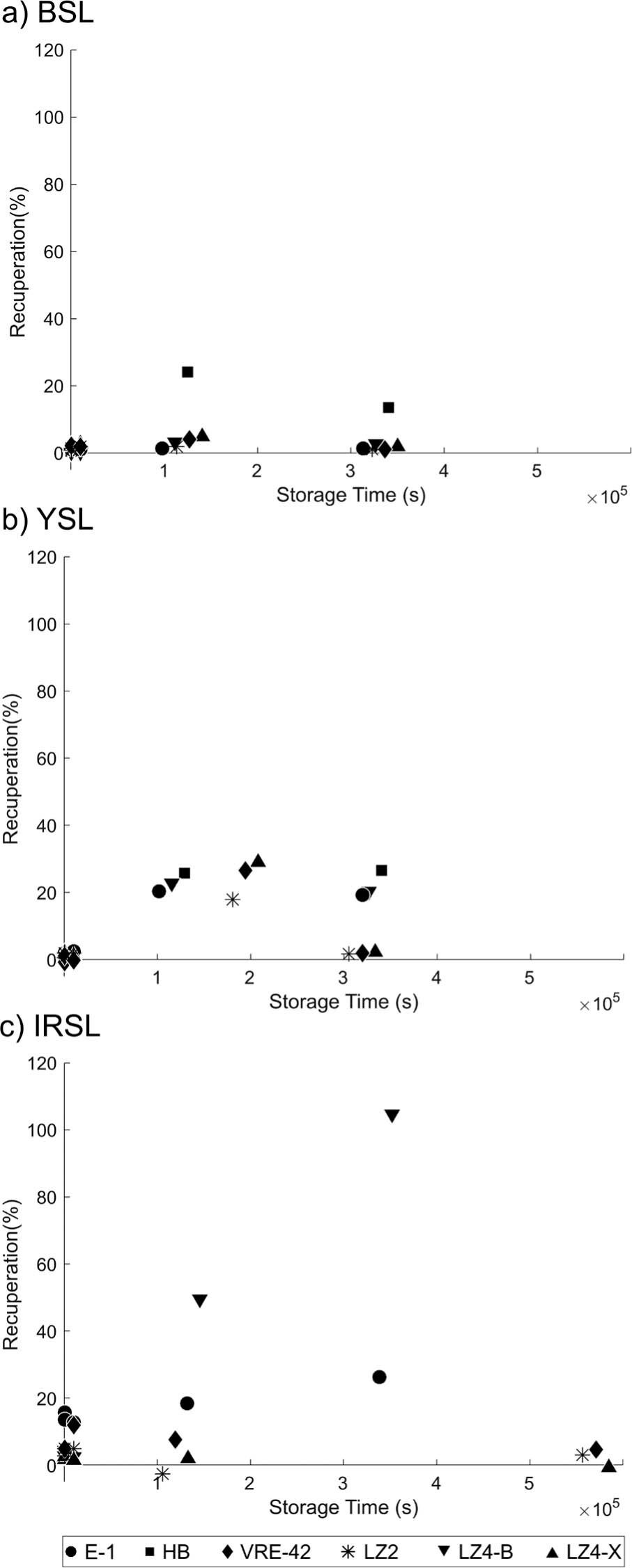
Fig 13
Dose recovery experiments: measured for each sample from BSL380, YSL380, and IRSL410 75 °C emissions. Growth curves (left, data jittered to aid visibility) and decay curves (right) are shown for each stimulation/detection combination. Both the signal measured directly after the Recovery Dose and the recuperated signal (post-bleach, five days storage) decay curves are shown. Test dose sensitivity changes are also presented (inset).
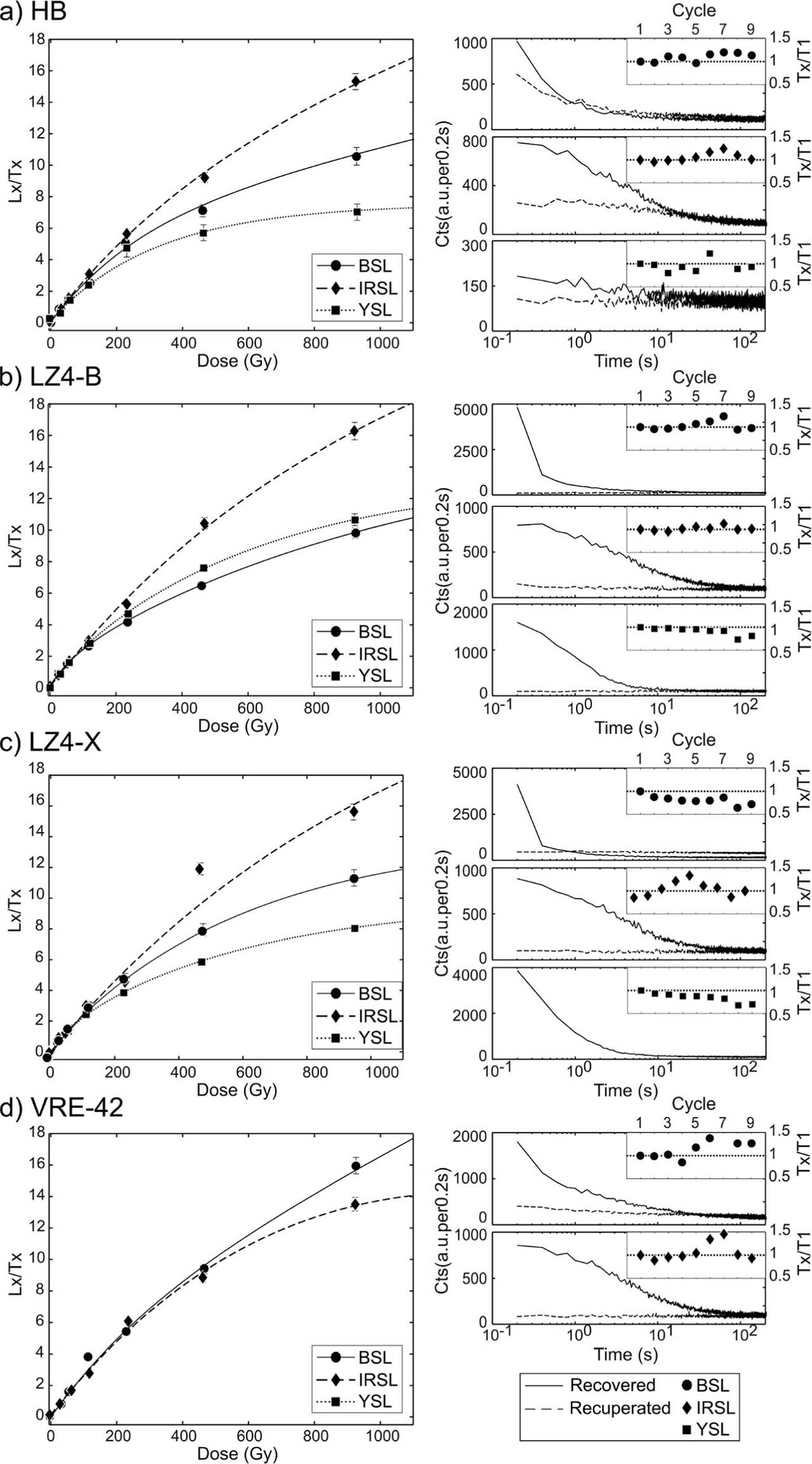
Table 4
Dose recovery results: each row corresponds to measurements made on one aliquot. The recycling ratio and zero-dose ratios are as defined in the text. Note that aliquots were not preheated prior to the five days zero-dose measurement. The recovered dose has been normalised by the given dose (116.0 Gy).
Finally, dose recovery experiments yield generally acceptable results. Recycling ratios and immediate zero-dose ratios were acceptable for all BSL and IRSL emissions; IRSL emissions tended to have higher immediate zero-dose ratio values, but all were under 5% of the induced ‘natural’ signal. Recycling ratios for the YSL measured aliquots were also acceptable, as were immediate zero-dose ratios for two of three aliquots; the third yielded a zero-dose ratio of 12.6 ± 5.5%. BSL380 and IRSL410 emissions recovered doses within one sigma of the given dose for all tested aliquots, with the exception of LZ4-X. Measurement of YSL emissions underestimated given doses by between 10% and 20%, though the recovered dose overlapped unity for one aliquot (HB) due to the magnitude of the error values for the dim signals. Irradiation-induced signals (‘growth curves’) are best fit with a sum of two saturating exponential functions in all but one case (HB YSL380), and all signals are still increasing at 1,000 Gy dose. The IRSL410 signal may typically saturate at higher doses than does the BSL380 and YSL380 signal, as this was the case for three of four tested samples. Sensitivity changes of nearly 50% are possible during SAR measurement, but it is not possible to draw any strong conclusions concerning patterns of sensitivity change from this limited data. Interpreting this data in the light of the fading experiment results is challenging, and further studies are necessary.
. Discussion
Luminescence characterisation of six intraplate olivine samples demonstrates that measurable TL and PSL signals can be induced via laboratory beta irradiation. TL peaks can be measured in both UV/blue and yellow/red bands, while UV and UV/blue PSL signals are observable with blue, yellow and IR stimulation from all samples. Dose recovery experiments are fairly positive with most aliquots, with acceptable recycling ratios and seven of eleven tested aliquots yielding a recovered dose within 10% of the given dose. Saturation levels are high, as luminescence signals are still increasing at nearly 1,000 Gy given dose. Considering typical dose rates for basalts <5 Gy·ka−1 (Tsukamoto et al., 2011; Rittenour et al., 2012; Shitaoka et al., 2014), such growth curves suggest that dates of at least several hundred thousand years could be measured.
Significant hurdles exist, however, if olivines are to be used as a natural dosimeter for luminescence dating. Both TL and PSL signals are relatively dim, given that many hundreds of grains were measured simultaneously and counting times of 0.2 s were used. TL peaks at temperatures >100°C were rarely observed at a given dose of ca. 50 Gy, and both high (464.5 Gy) and low (46.4 Gy) dose peaks are not well separated. PSL measurements of recuperation and fading indicate that sometimes significant charge populations are transferred from non-bleachable into bleachable traps during storage at room temperature. Indeed, though short-shine and dose recovery recuperation measurements suggest that this process may not be universal for all PSL signals and all samples, all fading experiments with the exclusion of E-1 BSL380 and YSL380 yield unexpected nonlinear signal decrease. This type of complex charge transfer invalidates one of the key assumptions of a De measurement protocol, i.e. the laboratory beta irradiation and aliquot preheating is an acceptable proxy for the storage over geological timescales. Finally, for the E-1 aliquots from which a fading rate could be calculated, extremely high g-values >40%/decade were obtained. Such values are too high to correct luminescence ages using standard tunnelling model equations (Huntley and Lamothe, 2001).
The luminescence characteristics noted in this study share some similarities with experimental results published previously; however, experimental protocols vary substantially, and results are therefore difficult to compare directly. Colin-Garcia et al. (2013) also note the presence of general TL peaks (no emission selection via filters) at ~100°C and below after laboratory irradiation of two samples (San Luis Potosí State, Mexico; Lanzarote, Canary Islands), however, non-ionizing UV irradiation was used. Takada et al. (2006) characterised three samples (USA, China, Pakistan), and also detected this low temperature peak in UV-blue TL. Additionally, however, they detect a fairly well separated peak at c. 190°C after irradiation (several tens to 124 Gy) and a peak at 275–310°C for doses >200 Gy. The first of these is present but very dim and not well-resolved in several of our samples, though it appears distinctly for our sample HB after a 464.5 Gy irradiation. The second, however, is only seen from sample E-1, and can be measured after both low and high irradiations. Koike et al. (2002) note both dim blue and strong yellow/red emissions for gamma-irradiated forsterite and natural olivines (Egypt) measured primarily at low temperatures (93–376 K). Comparable PSL characteristics are only available from two studies. In contrast to this study, Takada et al. (2006) find that BSL is generally dimmer than IRSL, but this is likely due to the discrepancy between the stimulation power: 15 mW·cm−2 and 370 mW·cm−2 for blue and IR LEDs, respectively. Examination of TL measured from an irradiated and IR bleached aliquot, however, is similar to the results reported here, with most of the trapped charge released by IR stimulation being stored in peaks <250°C but some released from up to c. 350°C. Jain et al. (2006) also measure a high saturation level of 4.3 kGy via a BSL340 SAR protocol from one aliquot of pure olivine (San Carlos, Arizona, USA), but this is a low-temperature (30°C) measurement after x-ray irradiation. Fading experiments for this olivine sample (250°C preheat, BSL340 @ 50°C) indicated much slower anomalous fading than the samples presented here, with only 20% of the signal lost after two to three days of storage. Given the paucity of samples and studies with which to compare and the variety of experimental protocols used, we suggest that significant further research is necessary to narrow down universal and sample-specific luminescence characteristics of olivines.
It is premature to draw any conclusions concerning the luminescence characteristics noted and the particular geochemistry, mineralogy and thermal history of the samples. Some possible correlations will be briefly mentioned, however, as avenues for future studies. Sample E-1 olivines are distinctive chemically, being the most differentiated, and they are emplaced within a ground-mass with unusual mineralogy compared to the other intraplate olivines studied. E-1 luminescence characteristics are similarly unusual, with a TL peak structure unlike any of the other characterised olivines (both low and high doses). E-1 olivines do share reliably detected PSL emissions with the other samples, but BSL bleaching efficiency is unusually enhanced, and BSL380 and YSL380 fading experiments yield very distinctive patterns. Given geochemical similarities between xenoliths LZ2 and LZ4-X, one might then expect these samples to share some luminescence properties. Interestingly, however, LZ2 and LZ4-X TL emissions are fairly different, while the basaltic olivines LZ4-B and xenolith LZ4-X are chemically dissimilar but TL emissions share peak wavelengths and emission temperatures. It is possible that the similarities between LZ4-B and LZ4-X are instead driven by the shared thermal history of the LZ4 olivines (Tinguatón eruption in AD 1824). Thermal history has been suggested as a fundamental driver of processes including fading rates (Guérin and Visocekas, 2015), sensitivity (Rendell et al., 1994) and presence/absence of particular TL emission peaks (Hashimoto et al., 1994; Ganzawa, 2010) in well-studied quartz and feldspar crystals. Of course, none of these studies relate particularly to olivines, therefore we must reason by analogy at this stage. Colin Garcia et al. (2013) have shown for two olivine samples (San Luis Potosí, Mexico and Lanzarote) that annealing olivines at 1100°C for one hour changes the texture of the crystal, observable under the scanning electron microscope, and may alter some of the peak centres for TL emissions (though this is after UV irradiation). Finally, one might expect that HB olivines, which have been subjected to repeated cycles of irradiation and bleaching as primary components of beach sand, should develop distinctive luminescence characteristics, potentially including significantly more sensitive PSL, as observed for quartz (Pietsch et al., 2008). HB olivines, though, are not unusual in either TL or PSL characteristics as measured in this study.
. Conclusions
Six olivine samples from intraplate settings have been geochemically and petrographically described and their luminescence signals (TL and PSL) have been characterised. This study has found that:
TL and PSL signals are dim to very dim,
All samples show a low temperature (90–100°C) emission peak in the UV/blue range, and five of six also have a low temperature yellow/red wavelength emission peak,
Measurable, distinct TL peaks at higher temperatures are rare (E-1), but where they exist, they are not quickly bleachable via PSL,
UV and UV/blue PSL emissions can be stimulated by blue, yellow and IR light,
Recuperation values may be quite high, and fading and recuperation tests suggest that complex charge transfer processes are underway in bleached olivines.
Further development of De measurement protocols for olivines will need to address these issues. It appears important to assess the olivine chemical composition and to determine their origin. Olivine xenoliths that have not equilibrated with the melt have a primitive composition, while phenocrysts incorporate a much wider range of elements possibly influencing trap availability and luminescence characteristics.