
. Introduction
Global climate changes have been drawing greatest attention in recent times, especially of the people living in the coastal areas, deltas and small islands. This is because one of the dominant ways in which climate change manifests itself is the rise/fall of sea level, which directly affects the coastal areas and delta formations worldwide. Scientific articles across the globe have shown records of sea level changes, as good indicators to look into the global climatic changes (Chappell, 1974; Hendey and Volman, 1986; Baxter and Meadows, 1999; Islam and Tooley, 1999; Devoti et al., 2004). With heavy concentrations of population and economic activities occurring in coastal regions, low lying deltas and islands, the perceived sea level rise has created the highest amount of concern in modern times (Dasgupta et al., 2007). Studies further suggest that hundreds to millions of people are likely to be displaced by the effects of sea level rise leading to serious economic and ecological damage and disequilibrium in the near future. Large changes in the sea level are not new and can be seen on a geological timescale as well, resulting from climate changes majorly as a consequence of glacial-interglacial cycles. During the last Interglacial approximately at 125 ka, when the north polar ice cap completely melted, the sea level was nearly 8 m higher than it is today (Dutton and Lambeck, 2012; Kopp et al., 2009). Bindoff et al. (2007) also showed based on tide gauge and satellite observations, a rise of about 1.7 mm/year in sea level over the 20th century, most likely a result of global warming over the same period. Therefore, there is an apparent connection between the changes in the climate and sea level, which should not be ignored when projecting the future. Apart from the past-future correlation, reconstructing sea level history is also significant as most of the geological records get generated by changes in the sea level. Studying such records not only give us clues about the environment/climate that has changed over geological time, but also give an insight into the sea level control on the geomorphological changes occurring over time. For instance presence of beach ridges, their geometry, elevation and orientation are good indicators of the past sea level variations, coastal morphodynamics and climate changes (Taylor and Stone, 1996; Kunte and Wagle, 2005). Sea level oscillations for Quaternary have been studied and recorded across the globe (Shackleton and Pisias, 1985; Stoll and Schrag, 1998; Antonioli et al., 2004). India has the sixth-longest coastline (eastern and western) in the world stretching over ~7500 km and is surrounded by the Indian Ocean, the Bay of Bengal and the Arabian Sea. However, the eastern coastal plains of India are much more significant for palaeoclimatic studies as they are wider, receive more rainfall, both from the NE and SW monsoons, and are more prone to cyclones/floods than their western counterparts. Palaeo sea level changes along the east coast of the Indian subcontinent have also been reconstructed using various proxies including relict coral reefs from the Bay of Bengal, dating of molluscs and marine shells (Rao et al., 1990; Rao and Rao, 1994; Vaz, 1996; Banerjee, 2000). In addition to the marine records, the archaeological and historical evidence also support the dynamic modifications of the east coast of India resulting from the global sea level transformations during the geological history. Offshore excavation carried out by Archaeological Survey of India (ASI) at Kaveripattanam- Poompuhar zone in Tamil Nadu shows that this important port town of early Chola Kings, was swallowed by the Bay of Bengal in ancient times (Rao, 1991; Gaur, 1997; Jayakumar et al., 2004). Despite the presence of marine and historical evidence, the continental records of sea level changes along the east coast of the Indian subcontinent are very limited and can be studied from channel and flood plain deposits, alluvial fans and deltas. Most of the major southern peninsular Indian rivers that originate in the western margin of the continent drain towards the eastern coastline, e.g. Kaveri, Godavari and Krishna rivers. These rivers receive both southwest and northeast monsoons and so respond by enhanced discharge and bed load, finally draining into the Bay of Bengal. As these rivers approach the Bay of Bengal, they form deltas unlike rivers draining westwards in the Arabian Sea and respond to sea level fluctuations by depositing or incising its bed (Singh et al., 2015). Their deltaic/coastal sedimentation is predominantly controlled by the 1) base level of the river controlled by sea level variations 2) hydrological parameters of the catchment like the discharge, sediment yield, etc. and 3) tectonics affecting the slope and subsidence of the basin area. Prolonged high discharge/humid phases are associated with sea level rise, increasing the base level of the river and thus forcing the river to aggrade, however, at the same time, prolonged humid phases reduce the sediment yield due to stabilized vegetation cover. Hence, the direct link of delta evolution with high discharge, sea level rises, tectonics or interplay of all these remains unclear. One of the objectives of this study is to contribute to understanding the link of climate in delta deposit.
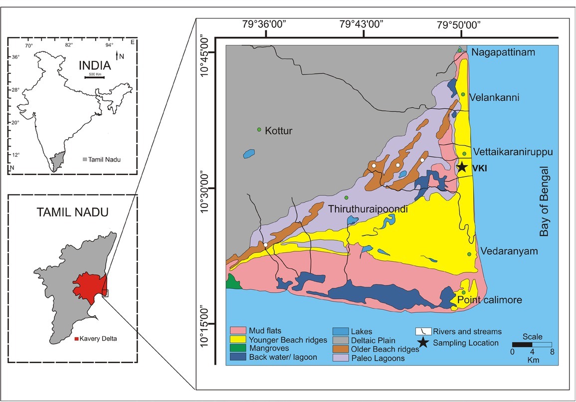
Kaveri is one of the major rivers of India that originates in the Western Ghats in Karnataka. It flows southeast over Mysore plateau and falls in Bay of Bengal flowing over the state of Tamilnadu covering an area of nearly 87900 km2 (Ramanathan et al., 1996; Singh and Rajamani, 2001). Kaveri delta looks like a flattened triangle, displays sets of beach ridge complexes and is a wave-dominated delta that has its origin located east of Tiruchirappalli. It is one of the major deltas of the Indian subcontinent that could be acutely affected by sea level rise. The sediment load carried by Kaveri is far less (1.5 million tonnes/yr) compared to the other peninsular rivers, like Godavari (170 million tonnes/yr), Krishna (4 million tonnes/yr), Mahanadi (15.7 million tonnes/yr), and Narmada (70 million tonnes/yr) rivers draining India peninsula (Subramanian, 1993). Few other smaller rivers like Pennar, Mahi and Brahamani also yield more sediment than Kaveri; however, their drainage areas are way less than Kaveri (Vaithiyanathan et al., 1988). Nevertheless, in a bedrock terrain like Kaveri’s, sediment yield could be high during end of an arid phase followed by the initiation of humid phase, i.e. during the transition of arid-humid phases similar to alluvial fan deposition (Singh et al., 2016, 2017). Hence, the deltaic deposition is expected to be high during the arid-humid transition and increase in sea level forcing the river to aggrade. Therefore, the Kaveri delta, as formed in a transitional environment between the river and sea gives various opportunities to look into the long term changes in the sea level and depositional environment (Singh et al., 2015).
Current work is an initiation of a major program to understand the geomorphic evolution of Kaveri delta, an archive of fluvial and shoreline activities. In order to do so, five cores were recovered, and the present study is based on one of them. The sediment core is analysed for optically stimulated luminescence (OSL) chronology, micropalaeontological studies, sedimentary and geochemical analysis to understand marine and deltaic fluvial responses to the palaeo sea level changes from the Kaveri delta and thus reconstruct past climate records. Morphometric analysis of the Kaveri basin displays its deltaic region to be tectonically stable in recent and in geological past (Kale et al., 2014). This study, therefore, introduces a classic stratigraphic question about the control of sea level in a wave-dominated deltaic environment.
. Geology and geomorphology of the study area
Kaveri basin is majorly underlain by the Archean-Proterozoic crystalline rocks constituting charnockites, gneisses and granites (Sharma and Rajamani, 2001; Alappat et al., 2010). Toward its east, the deltaic part is covered by quaternary alluvium with exposures of Cretaceous sediments (Uttatur, Ariyallur, Tiruchirappalli-foramations) and sandstone (Cuddalore formation) of Mio Pliocene age (Alappat et al., 2010). The quaternary sediments consist of the fluvial sediments, middle Holocene beach ridges, late Holocene sand dunes (Alappat et al., 2010; Kunz et al., 2010). The present-day river flows as river Coleroon through the northern channel of the delta. The deltaic part of the basin receives mainly NE monsoon (June to September). However, the SW monsoon brings much sediment to the delta from the uplands (Alappat et al., 2010). The suspended sediment load of the river is predominantly derived from relatively stable Precambrian shield rocks (granites and gneisses), covering almost 80% of the drainage area of Kaveri. This makes the weathering process insufficient accounting for the low sediment load carried by the river, as mentioned. The average annual runoff of the basin as compared to the other non-Himalayan rivers like the Godavari (111 km3), Krishna (78 km3), Mahanadi (67 km3) and the Narmada (46 km3) is also significantly low about 21.4 km3 (CWC 2012), implying low unit discharges of river Kaveri. The coastal geomorphic map of the study area shows the presence of landforms like younger and older beach ridges, palaeo lagoons, mangroves, tidal flats, mudflats, sand bars in the study area (Fig. 1). The east coast of Tamil Nadu features several beach ridges, varying from few meters to several tens of meters. The geometry of the beach ridges observed showcases that there had been a shift in the coastline responding to the changes in the past climate.
. Methodology
Sampling location and Collection of samples
The palaeo beach ridges were the target areas to obtain sediment cores of 25 m depth each. Three sets of beach ridge complexes were observed in the field as well as by the satellite images that showed the diversified geomorphology of the area under observation. The nose point shape of the delta formed by two perpendicular sets of beach ridges and the third one is oblique to that taken for study. A 25 m long core (VKI) under the present study was collected from Vettaikaraniruppu (N 10° 33.208'/ E 79° 50.127'), situated 2.6 km onshore from the present coast of Tamil Nadu, east coast of India (Fig. 1). The present altitude of the coring site is 7.2 m above mean sea level (MSL). Geomorphology revealed sets of beach ridges indicating the palaeo shorelines. Core samples were excavated by calyx core drilling with low rpm. Undisturbed dry sample was taken with dry drilling so that the core does not get washed away. Double tube core barrel was used with an inner PVC tube, to prevent the core sample from collapsing and to protect them from daylight exposure, which is a necessary condition for luminescence dating. In the drilling operation, water was used for cleaning borehole and mud water for loose formation so that the hole did not collapse. The core was then cut into two halves at Core cutting facility (National College (Autonomous), Tiruchirappalli, Tamil Nadu, India). One of the cut halves of the core was used for micropalaeontological studies, sediment analysis and luminescence chronology. Fifty subsamples (VKISS 1 to VKISS 49) were collected at every 0.5 m for micropalaeontological studies and grain size analysis. Thirteen samples (VKI 2 to VKI 14) were collected at each 1.5 to 2 m approximately for luminescence chronology. Topsoil sample up to 1.5 m depth was not taken in the core to avoid contamination from bioturbation.
Core description
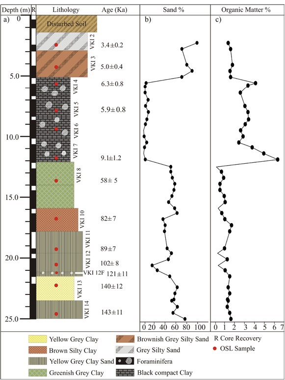
VKI core shows lithological variations at increasing depths. A simplified diagrammatic representation of the VKI core is given in Fig. 2. The uppermost part of the core (1.4–5.1 m) is majorly composed of silty sand (VKI 2, VKI 3) followed by a thick distinct sequence of black (organic-rich) compact clay (VKI 4, VKI 5, VKI 6, VKI 7) extending to a depth of 12.0 m. Micropalaeontological study shows the presence of foraminifera (discussed in 4. Results – Micropalaeontological analysis) in this layer. It is then followed by ~4.0 m thick deposition of slight greenish-grey clayey sand that continued till 16.0 m at increasing depths (VKI 8). Brown sandy clay was observed from 16.0–17.8 m (VKI 10) followed by yellow grey sandy clay at a depth of 21.5 m depth (VKI 11, VKI 12). However, within this layer, at a depth of 21.0–21.5 m (VKI 12F) presence of foraminifera is observed. The sand abundance in this layer is nearly 20%. Further down, yellow grey clayey sand was observed continuing until the bottom of the 25.0 m core (VKI 13 and VKI 14). Seven lithological units in the VKI core were visually identified and dated. The core represents various stages of fluvial and marine activity in the region.
Fig. 2
(a) Chronostratigraphic cross-section of the VKI core, taken along the NS trending palaeo beach ridge parallel to the present coast. (b) Depth vs sand (%) graph showing a distinct change in the sediment type down the core. (c) Depth vs organic matter (%) graph showing variation in the total organic matter content down the core.
Micropalaeontological analysis
10 g of sediment was taken from each sample interval at 0.5 m for foraminifer’s separation (VKISS 1 to VKISS 49). For the entire 25 m core, a total of 50 samples were analysed. The samples were dispersed in sodium hexametaphosphate solution to get rid of the agglomeration of particles, washed in running water through ASTM 230 (mesh size 63 μm) no. sieve and oven-dried below 50°C. Floatation method using CCl4 was adopted to separate foraminifera in the remaining sample. Samples were spread evenly on the picking tray with numbered grid and foraminifera were examined through a binocular stereo microscope. Total abundance of planktic and benthic foraminiferal specimens and stress markers per 10 g were calculated. Our counts included broken specimens along with full specimens. However, the abundance of broken specimens was low leading to minor overestimation of the counts. Depth wise variations in foraminiferal abundances in the core are given in Table 1.
Table 1
Table showing relative abundance of foraminifera: benthic, planktic and stress markers down the VKI core.
Sedimentological and geochemical analysis
10 g of sediment was taken at every 0.5 m for grain size estimation. Wet sieving was carried out using ASTM 230 sieve to wash away the mud particles (< 63 μm; silt and clay size). The retaining sand sample was used to estimate sand percentages.
Total organic matter was estimated by Walkley and Black titration method, widely used for organic matter analysis in sediments. The method is based on the oxidation of organic matter by potassium dichromate (K2Cr2O7)-sulfuric acid mixture followed by back titration of the excessive dichromate by ferrous ammonium sulfate (Fe(NH4)2(SO4)2*6H2O) (Walkley and Black, 1934, Walkley, 1947; Jackson, 1958). 1 gm of dried samples taken at every 0.5 m in the core was treated with 10 ml of 1N K2Cr2O7 followed by addition of 20 ml of concentrated sulfuric acid. The mixture was gently stirred and left in the fume cupboard at room temperature for 30 minutes. It was then diluted with 200 ml of Milli-Q water. The excess of dichromate was back-titrated with 0.5N ferrous ammonium sulfate solution; the endpoint was the colour changes from mixed green to brilliant green. The titrate value was recorded. Blank titration of the acidic dichromate with ferrous ammonium sulfate solution was performed using the same procedure with no sediment added. As given by Jackson, 1958 the organic matter content (%) in the samples was calculated as 10×(1-(S/B))×0.67, where B is the volume of ferrous solution used in the blank titration and S is the volume of ferrous solution used in the sample titration.
Optically Stimulated Luminescence (OSL) Dating
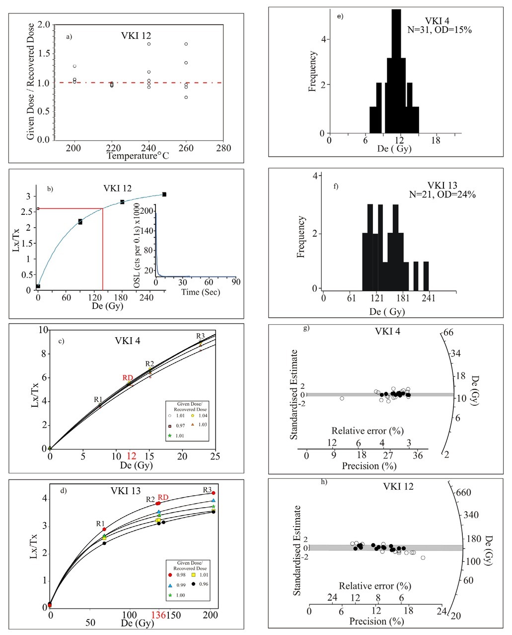
OSL dating technique was used to provide a robust chronological framework to the core. OSL dating provides an estimate of last daylight exposure of sediments, thus giving last burial ages (Aitken, 1998; Huntley et al., 1985). Thirteen samples (core tubes of length 10 cm each) from different lithological units were cut from the core for luminescence dating. All the processes were carried out in subdued red light conditions. The middle part of core tubes (light unexposed) was processed by treating the sample with 10% HCl and 30% H2O2 to remove carbonates and organics respectively. Selected grain size fraction (90to 150 μm diameter) was isolated by wet sieving. From the sieved fraction, quartz and feldspar grains were separated from each other using freshly prepared sodium polytungstate solution (ρ=2.58 g/cm3). The quartz grains obtained were further etched with 40% HF for nearly 80 minutes to remove the alpha dose affected layer (assumed to be 15 ± 5 μm) and then treated with 30% HCl for nearly 30 minutes to remove fluorides formed in this reaction. Quartz grains were then mounted on stainless steel cups as monolayer using SilkosprayTM silicone oil. Luminescence measurements were made on Lexsyg smart TL/OSL reader (Freiberg Instruments, Germany). The instrument is equipped with blue-light-emitting diodes (LED) arrays of wavelength 458 ± 10 nm, detection window consisting of a combination of optical filters Hoya U340 and Delta BP 365/50 EX mounted on a solid-state photomultiplier tube (PMT) along with 90Sr/90Y beta source (Richter et al., 2013). The beta source delivered a dose rate of 0.15 Gy/s. Feldspar contamination was tested using infrared stimulated luminescence (IRSL). No significant IR signals were observed confirming the purity of quartz extracts. To obtain the equivalent doses (De) from each sample, the Single Aliquot Regeneration (SAR) protocol (Murray and Wintle, 2000) was followed. Preheat plateau test was conducted on VKI 12 for temperatures between 200°C to 260°C, hold time for 20 sec and a cut heat of 160°C. Results suggested 220°C for 20 sec as the most appropriate preheat temperature and thus was used for further luminescence measurements (Fig. 3a). Dose response curves of all the samples except VKI 13 and VKI 14 were fitted with a single saturating exponential function. For VKI 13 and VKI 14 sum of two saturating exponentials gave better dose estimates. For higher doses near saturation, the dose response is well represented by the sum of two saturating exponential functions (Murray et al., 2007; Pawley et al., 2010; Timar-Gabor and Wintle, 2013). Dose recovery test was performed on two samples, VKI 4 (younger sample) and VKI 13 (older sample). Laboratory doses of 12 Gy and 136 Gy were given and recovered from 5 bleached aliquots of these samples respectively. The ratios of the given dose/recovered dose were 0.99 ± 0.02 and 1.00 ± 0.02 respectively, and even the older age is well recovered. This procedure suggested that the SAR protocol can recover the laboratory doses, thus validating the reliability of the protocol used (Fig. 3c, 3d)).Aliquots having recuperation <5%, test dose error <10% and recycling ratio within 10% of unity were selected for calculating the De. In addition to this, for doses near saturation (for samples VKI 13, 14), only the values from aliquots with natural sensitivity corrected OSL response (Ln/Tn) less than the saturation value obtained from the dose response curve were selected (Thomsen et al., 2016). The values near saturation have relatively higher errors owing to the exponential nature of the curve. During computation, all these values are considered along with their errors. However, the De estimation taking error into account will weigh the values according to their errors with values having lesser error getting more weight. This will lead to biasing of the result towards the lower De values. Thus, the quoted ages for VKI 13 and 14 provide lower bound to the true ages, and the actual ages could still be on the higher side (Galbraith and Roberts, 2012). Central age model (CAM) was used for estimating the doses as the overdispersion (i.e. the relative spread in De values remaining after allowing for measurement uncertainties) in the all the samples remained less than 40%. (Galbraith et al., 1999; Bailey and Arnold, 2006) (Fig. 3e, 3f). CAM takes into account any overdispersion in the dataset while determining the weighted mean and its standard error (Galbraith et al., 1999; Galbraith and Roberts, 2012). In order to calculate the dose rates, the outer ~2.0 cm of sediment were scraped off at both ends of the core tubes (due to chances of light exposure during cutting) and used for the analysis of radioelements concentration of uranium, thorium and potassium determined by an inductively coupled plasmamass spectrometer (ICP-MS). Moisture content in marine samples (samples with presence of foraminifera) was taken as 50 ± 25 (%) and 20 ± 10 (%) for non-marine sediments (absence of foraminifera in the samples). Final dose rate estimations were made using DRAC v1.2 online software available (Durcan et al., 2015).
Fig. 3
(a) Preheat plateau test of VKI 12 shows 220°C as optimal preheat temperature (b) Laboratory generated dose growth curve; (inset) BSL shine down curve of VKI 12. (c, d) Dose recovery tests of VKI 4 and VKI 13 respectively (RD = Recovered doses), R1, R2, R3 are the regenerated laboratory doses shown in different colours for 5 different aliquots, laboratory doses given are shown in red. (e, f) Frequency histograms of VKI 4 and VKI 13 showing < 40% overdispersion. (g,h) radial plots of the measured doses of samples (VKI 4, VKI 12) respectively.
Two organic-rich sediment samples VKI 4 (5.75 m) and VKI 7 (11.85 m) were also AMS radiocarbon dated to check with the OSL chronology. Measurements were made using Accelerator Mass Spectrometer (AMS) facility available in Inter University Accelerator Centre (IUAC), New Delhi (Kumar et al., 2015; Sharma et al., 2019).
. Results
Micropalaeontological analysis
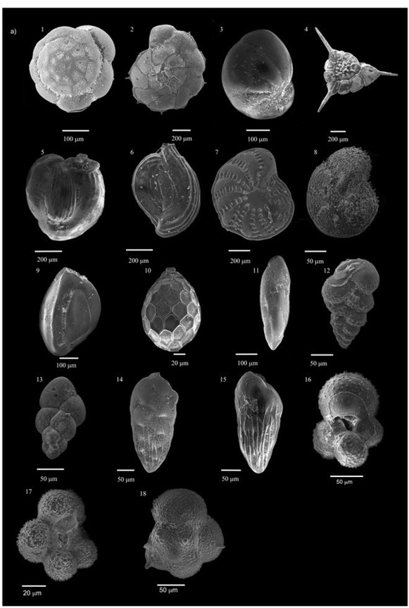
Presence of microfossils (benthic and planktic foraminifera) is observed in two distinct sections of the core; (section 1) 5.6 m to 10.9 m depth (VKI 4,5,6,7) and (section 2) 21.0 m to 21.5 m depth (VKI 12F). Foraminifera’s signatures indicate the sediments were deposited as a result of marine transgression in the geological past. The planktic foraminifera’s abundance varied from 30% to 60% from 5.6 to 10.9 m depth, unlikely to occur in the beach or marginal marine environment. Certain infaunal benthic species (stress markers) were also identified from section 1. Infaunal benthic reflect the effect of oxygen stress in a biotic system (Mazumder and Nigam, 2014). Such a high abundance of plankticforaminifera and presence of infaunal species was not observed in section 2. Fig. 4 shows scanning electron microscope (SEM) images of various depth markers, stress markers and the planktic foraminifera observed in the VKI core.
Fig. 4
Benthic foraminifera: 1 – Ammonia beccarii, 2 – Pararotaliaozawai, 3 – Nonionellinalabradoricum, 4 – Asterorotaliatrispinosa, 5 – Flintinabradyana, 6 – Spiroculinaantilluram, 7 – Elphidiumadvenum, 8 – Elphidiumsp, 9 – Triloculinatrigonalla, 10 – Oolinahexagona, 11 – Fursenkoinacomplanta (stress marker), 12 – Bolivinapseudolobata, 13 – Buliminagibba (stress markers), 14, 15 – Bolivinastraitula (stress markers). Planktic foraminifera: 16 – Globigerina bulloides, 17, 18 – Globigerina sp
Sedimentological and geochemical analysis
The relative abundance (%) of sand (> 63 μm) and silt-clay (< 63 μm) sediments from fifty subsamples (VKISS 1 to VKISS 49) are shown in Fig. 2b. Sand is dominating (70–80%) in the top portion of the core from 1.4 m to 5.1 m. Sand abundance declines to ~10% and silt-clay dominates (90–90.5%) in the marine sediments present from 5.6 to 10.9 m. Beyond this, there is a significant decline in silt-clay abundance and increase and subsequent rise in the sand abundance. Further down the contribution from both the sediment types (sand and silt-clay) remains nearly 50% with minor variations till the bottom of the core. Only when the marine sediments reappear at 21.0 to 21.5 m, silt-clay gets abundant (73–83%).
The organic matter is also high in marine sediments (5.6 to 10.9 m depth), ranging between nearly 2.5–6% (Fig. 2c). However, the rest of the core showed organic matter ranging between 0.3–1.5%.
OSL Chronology
Quartz grains obtained from all thirteen samples (except VKI 4, 5 and 6) have shown high sensitivity with luminescence counts reasonably high (~1.5×10⁵ counts per the initial 0.1 seconds of the shine down curve for 1 mm small aliquots). Comparatively, luminescence signals in VKI 4 and VKI 5 were much lower, ranging from few hundreds to few thousands per the initial 0.1 seconds of the OSL decay curve. VKI 6 has shown significant low sensitivity and did not have enough and detectable blue stimulated luminescence (BSL) signals. VKI 4, 5 and 6 are from the marine section of the core with the presence of microfossils, and thus there is a clear separation of sensitivity in fluvial sediment and sediment of marine origin. The older, pre-Holocene terrestrial sediments were observed to be approx. 102 times brighter than the Holocene marine sediments. The dose rates of the samples were low (Table 2), and quartz has not shown saturation even at doses as higher as 200 Gy. (Observed from the dose response curve and dose recovery test of older samples), that helped in the dating of older sediments easily using quartz (Fig. 3, Table 2).
Table 2
OSL age table of samples analysed from VKI core showing various parameters for age calculations.
The youngest ages in the core from the top-most grey silty sand and brownish-grey silty sand units are estimated to be 3.4 ± 0.2 to 5.0 ± 0.4 ka at a depth of 2.6 m and 4.4 m respectively. Further down along the core, the thick continuous sequence of marine sediment encountered is dated 6.3 ± 0.8 ka at 5.8 m, 5.9 ± 0.8 ka at 8.0 m and 9.1 ± 1.2 ka at 11.9 m. The radiocarbon ages at 5.8 m and 11.9 m were calculated to be 7932–7786 cal BP (1σ) (Lab code: IUACD#16C436) and 8700–8484 cal BP(1 σ )(Lab code: IUACD#16C437) respectively showing close accordance with the OSL ages and validated the application of OSL dating technique to marine sediments. These ages are calibrated using OxCal software with int. Cal 13 calibration curve (uncalibrated ages are 7004 ± 60 and 7817 ± 60 at 5.8 m and 11.9 m respectively). OSL sample was retrieved from the next encountered greenish-grey clayey sand at a depth of 13.8 m and was dated 58 ± 5 ka. Next brown sandy clay at 16.9 m depth was dated 82 ± 7 ka. Two OSL samples were obtained at 19.4 m and 20.8 m from the underlying yellow-grey sandy clay unit and dated 89 ± 7 ka and 102 ± 8 ka respectively. Fine pelagic unit observed within the yellow-grey sandy clay at 21.2 m was dated 121 ± 11 ka. Towards the bottom of the core the yellow-grey clayey sand unit was dated at a depth of 22.8 m and 24.7 m giving age estimates of 140 ± 12 ka and 143 ± 11 ka respectively. Detailed OSL chronology of the VKI core is given in Table 2, Fig. 2a.
. Discussion
The low annual sediment load and low discharge of Kaveri lead to a very low rate of sedimentation in the deltaic environment. However, the sediment load and the discharge could be temporarily high during intense humid phases following the arid phase, a suitable climatic optimum for delta deposition in such setting.
Relative sea level variations for late Pleistocene and Holocene indicate relative stabilization of the sea level during the last 5–6 ka (Aloïsi et al., 1978; Dubar and Anthony, 1995; Morhange et al., 2001). Although few studies based on global isostatic modelling tentatively suggest a sea level rise of 2 m in the last 6000 years (Nakada and Lambeck, 1988; Lambeck, 1993). The topmost depositional part of the core provides an age of ~3.4 ka indicating a higher sea level stand or high discharge or both on the southeastern coast of Tamil Nadu region. A similar study in this region by Ramasamy et al. (1998) using C-14 dating and Thomas (2009) using OSL of beach sediment in the southeastern coast of Tamil Nadu suggests higher sea level stand during this period. In addition, due to increased insolation, monsoon intensified at 3.6 ka and continued till 2.5 ka in the associated basins studied. This conclusion was based on pollen records in Pookot lake sediment core (Bhattacharyya et al., 2015) and channel sediment studies in Palar basin in the north of Kaveri delta (Resmi et al., 2016). The high monsoon phase enabled the river to carry relatively higher sediment load than its usual that got deposited in its deltaic region due to the suggested rise in sea level.
Another depositional event occurred around 5.0 ± 0.4 ka, (VKI 3; Fig. 2) suggesting another sea level high-stand/high river discharge during this time. Based on radiocarbon dating from the east coast of India, Banerjee, (2000) also concluded that the sea level 5500 years ago was 2 m higher. Similarly, the radiocarbon dates of coral colonies along the adjacent south-west coast of Sri Lanka also indicate sea level high stand during 6170–5100 years (Kattupotha and Fujiwara, 1988). Monsoon intensification was again observed between 6.5 ka to 5.5 ka ago. Drier phases were reported for 5.5 ka to 4.1 ka and from 2.3 ka to present based on δ18O and G. rubber record from the marine sediment core retrieved from the eastern region of Bay of Bengal (Achyuthan et al., 2014). The drier phases that prevailed during 5.5 to 4.1 ka and post 2.3 ka are evident by no significant sedimentation in the deltaic region under study. Thus, it is well observed that the depositional records in the past 6000 years correlates well with the early reported mid to late Holocene sea level high-stands, humid phases in the Indian subcontinent and supports the modelled tentative records of sea level rise during 5 ka and 3 ka. Although increased monsoon intensity prompted the discharge and sediment yield of the river to increase, sediment deposition in the delta was a result of the river’s attempt to attain new equilibrium in response to the increased sea level, thus modifying its base level. Thus, rivers like Kaveri with low discharge and low sediment yield preserve strong sedimentation records in its delta during major climate changes when the sea level is increased, and the monsoon gets intensified. Since there is no direct evidence of sea level transgression (lack of foraminifera in the sediment), it can be suggested that during ~5 ka and ~3 ka, sea level rise was not very high (sea level rise of around 2 m around 5500 years on east coast of India, as suggested by Banerjee, (2000)) but it led to the fluvial deposition at the studied site. This indicates the strong control of sea level on the depositional pattern of Kaveri delta. During ~9 ka the sea level increased, reaching the onshore sampling site and remained there for another 3 ka with some fluctuations. This is evident by the deposition of ~6 m thick sequence of fine-grained pelagic sediments comprising benthic and planktic foraminifera, during ~9–6 ka. Variations in the planktic abundances (30–60%) provide evidence of several minor phases of transgressions and regressions within the major sea level oscillation at 9–6 ka. High organic matter content ranging from 2.5–6% and the presence of certain infaunal benthic genera (Bolivina, Bulimina, Fursenkoina) indicate oxygen-depleted conditions during this time phase. 9–6 ka is reported as a high humid phase resulting from the increased solar radiation during the same period. This was the period of mid-Holocene monsoon maxima, and sea level was higher than at present, very well reported worldwide (Prell and Kutzbach, 1987; Kar et al., 2014) (Fig. 5). Great river influx in the Bay of Bengal during 9–6 ka established oxygen stressed conditions that led to ~5 m thick pitch black, compact, pelagic, organic carbon-rich sediment accumulation in the core. It is suggested the pitch black, pelagic, organic-rich sediment be sapropel deposition associated with the early to mid-Holocene monsoon maxima in the Kaveri delta. Similar sapropelic depositions are also recorded from the eastern Mediterranean basin and the Adriatic Sea during ca. 9.5 ka-6.5 ka (Prell and Kutzbach, 1987; Rohling, 1994; Ariztegui et al., 2000; Kallel et al., 2000; Emeis et al., 2003; De Lange et al., 2008). Sapropel formation reflects short-term variations in oceanographic conditions (stratification and anoxia) (Ariztegui et al., 2000). Further investigation of the offshore basin could result in better correlation. The current study depicts that this transgression during MIS 1 (9–6 ka) was most distinct and greatest in comparison to the other late Quaternary sea level highs in the Tamil Nadu coast where marine signatures were absent above MSL. However, only during the beginning of MIS 5 (~121 ka), foraminiferal signatures are again observed above the present MSL. This indicates that the Bay waters once again transgressed, up to the site of observation. Banerjee, (2000) reported a relative rise in the sea level of about 4.5 m above the low tide level along the east coast of India during the late Pleistocene (128 ± 1 to 116 ± 1 ka). Quaternary sea level curve also depicts sea level higher than the present during this period (Fig. 5). The thickness of the marine deposition during ~121 ka was way less (~0.5 m), relative to the ~5.3 m pelagic sediment deposition during 9–6 ka along with less abundance of foraminifera (<15 foraminiferal specimens/10 g), in the study area. This suggests the effect of sea level transgression during early MIS 5 was less pronounced and short-lived as compared to the early to mid-Holocene transgression. The grain size analysis of the marine sediment deposited during the Holocene transgression maxima (9–6 ka) and late MIS 5 transgression (~121 ka) depicted depositions occurred in quieter, deep water conditions, as silt and clay deposition dominated (Gross, 1972).
Fig. 5
Summary of sea level fluctuations over the last 150 ka. The black bars represent durations of deposition in the core. The depositional periods in the core matches closely with sea level highs. The grey line depicts the present sea level. (Modified after Gibling et al., 2005; Waelbroeck et al., 2002; Singhvi et al., 2012).
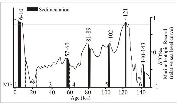
OSL chronology of the core suggests that further deposition occurred at ~60–57 ka (MIS 3), ~87–81 ka (MIS 5), ~100 ka (MIS 5) and~143–140 ka (MIS 6). These depositional units are non-marine as no marine signatures (foraminifer’s evidence) were observed. However, interestingly the depositional periods of these non-marine fluvial units coincide well with the sea level rise as reported by Shackleton and Pisias, (1985), Gibling et al. (2005), Waelbroeck et al. (2002) during the late Quaternary(Fig. 5). This suggests that the sea level rise along the east coast of India is following the late Quaternary changes in the sea level. Although due to the absence of direct marine evidence (foraminifera) in these units it can be concluded that during these periods the sea waters did not transgress up till the onshore sampling site. Instead, the effect of the sea level rise is observed as a fluvial deposition. Previous literature suggests that monsoon, in general, was high during these above-mentioned sea level peak periods as a result of increased summer solar radiation in the northern hemisphere (Prell and Kutzbach, 1987). This resulted in high discharge in the river enabling it to carry more than its usual sediment. The ample sediment carried by the river got deposited in the delta because of the river’s adjustment to the new base level due to the rise in sea level, instead of getting deposited into the sea. Drier phases/ glacial periods, on the other hand, were accompanied by high rates of sea level fall, low discharge and low sediment load of the river and consequently insignificant sedimentation was registered as inferred by the depositional breaks in the subsurface core studied hereby (Fig. 5). This study proposes high deposition in Kaveri delta coast concurred with humid-arid climatic transitions and increased sea level due to increased monsoon/glacial melting during the last 150 ka. In contrast, during drier climatic phases or glacial periods, absence of sedimentation is observed due to low sediment availability in the catchment as well as very low discharge in the river. Although the record of ameliorating monsoon during the transition phase of Last Glacial Maxima (LGM) to intense humid phase is missing in the present core, it could be due to a complete shift of the channel due to heavy sediment load as the channel tends to shift in a deltaic environment. In addition, a hiatus in sedimentation is also observed after ~57 ka and deposition occurred only at ~9 ka. This depositional break could also be a result of non-continuous nature of sedimentation in deltas or could be attributed to the continuous lowering of the sea level with minor fluctuations post ~60 ka (early MIS 3) until the rise of sea level at ~9 ka (MIS 1) (Fig. 5). It requires studies from a few more cores to complement the sedimentation gaps found in the current study. This study is in progress, and a complete picture of deltaic sedimentation is expected in the near future. A similar kind of response of the Kaveri was observed by Singh et al. (2015); however, the study was limited to Holocene, and no marine signatures were observed in the study. Thus, based on the robust chronological, micropalaeontological and sedimentological study of the onshore subsurface sediment core it is evident that even minor climatic changes have affected the sea level in the Tamil Nadu coast; however, such fluctuations are not always accompanied by marine signatures onshore. Instead, the river is observed to have responded to these minor fluctuations by depositing sediments in its deltaic region. Sea level rise along the east coast of India is also observed to be following the late Quaternary changes in the sea level.
. Conclusions
Current work shows the dominant control of sea level variations on deltaic/coastal stratigraphy, considering the variations in the climatic changes that can affect the hydrological parameters, i.e. the discharge and sediment load of the river. Kaveri delta is observed to respond to even relatively minor sea level fluctuations along the Indian east coast over last 150 ka. Thus, this paper discusses the strong control of marine and fluvial activities in Kaveri delta formation and coastal sedimentation, highlighting the importance of fluvial, deltaic sedimentation as an archive to past sea level changes, even in the absence of direct marine records. The current study is supplemented by robust chronological framework, sedimentary and micropalaeontological analysis.
Vigorous chronology of the depositional units observed in the core concluded significant sedimentation occurred at around ~3.4 ka (MIS-1), ~5.0 (MIS-1) ka, 9–6 ka (MIS-1), 60–57 ka (MIS 3), 89–81 ka (MIS 5), ~102 ka (MIS 5) and 143–140 ka (MIS 6) in the Kaveri delta, correlating well with past humid-arid climatic transitions and sea level high-stands. The varying thickness of these depositional units and absence/presence of micropaleontological signatures suggest their varying impacts on the Tamil Nadu coast from one another.
A major sea transgression occurred during 9–6 ka, also reported from other parts of the world and is observed in the study area by the presence of foraminifera. The variation in the planktic foraminiferal abundance (%) provides evidence of several minor fluctuations in sea level within the major early to mid-Holocene transgression (9–6 ka).
In addition to the early Holocene sea level fluctuation, sea level rise is also observed during at ~121 ka (MIS 5) evident from the presence of foraminifera’s signatures present above MSL. However, the most pronounced sea level transgression was the early to mid-Holocene maxima followed by the early MIS 5. The other sea level high-stands observed in the core were even less pronounced in the southeastern India coast for the sea to transgress ~2.5 km onshore.
The fluvial depositional units and marine records depict a clear response between monsoon/arid-humid transition phases and sea level changes. Thus this study concludes strongly, the importance of fluvial responses in reconstructing the past sea level fluctuations as observed from the river’s depositional mode on the base level increase, linked with sea level rise, in a deltaic environment with no significant tectonic control.
The close correlation between the OSL ages and radiocarbon ages of the marine sediments indicates the reliability of OSL dating technique for marine sediments.