
. Introduction
Loess can be simply defined lithogenetically as a terrestrial silt deposit of aeolian provenance (Pye, 1987, 1995; Follmer, 1996; Smalley et al., 2001; Smalley and Jary, 2004). Loess-paleosol sequences (LPS) are an exceptional source of palaeoclimate data, providing an indirect record of changing environmental and climatic conditions that existed during loess deposition and early diagenesis (Muhs, 2007, 2013; Rousseau et al., 2013; Schaetzl et al., 2018). This is due to the lithological and structural characteristics of LPS.
The Northern European Loess Belt (NELB) extends from southern Great Britain to northern France, Belgium, Netherlands, Germany, Ukraine and Russia (Różycki, 1991; Pécsi and Richter, 1996; Smalley and Jary, 2005; Haase et al., 2007), includes loess in Poland. In the foreground of the massive Pleistocene Fennoscandian ice sheets, the NELB was formed (Lehmkuhl et al., 2021). The dynamic changes in Pleistocene periglacial settings significantly impacted the formation of the Late Pleistocene LPS in Poland, which developed over relatively brief but locally intense sedimentation periods (Jary and Ciszek, 2013).
Maruszczak (1991) developed the first complex loess stratigraphic scheme in Poland using the findings from thermoluminescence (TL) dating. Recent optically stimulated luminescence (OSL) and radiocarbon dating conducted in Gliwice have been used to verify the Late Pleistocene part of this scheme (Moska et al., 2011, 2012, 2015, 2017, 2018, 2019a, 2019b). The study's findings made it possible to correlate Poland's Late Pleistocene LPS with the unified loess stratigraphic scheme as suggested by Marković et al., (2015).
According to Jary et al., (2002), loess in SW Poland creates a discontinuous cover having a range of thickness with stratigraphic and physical characteristics (Fig. 1A). The Niemcza-Strzelin Hills are a site to the most representative LPSs, which span the most recent interglacial-glacial cycle. The greatest example is the Biały Kościół LPS (Jary, 2007, 2010; Moska et al., 2011, 2012, 2019a; Jary et al., 2016; Zöller et al., 2022). It has well-developed S1, L1LL2, L1SS1, L1LL1 and S0 litho-pedostratigraphic units and reliable chronology.
Fig 1.
(A) – Loess distribution in SW Poland (modified after Jary, 2010); (B) – location of the Zaprężyn LPS.
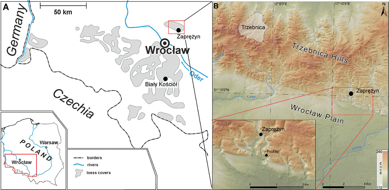
The northernmost loess region in SW Poland is located in Trzebnica Hills, and it is just around 70 km from the front of the ice sheet during the Last Glacial Maximum (Marks, 2012). Late Pleistocene loess of this region has been recognised in the Trzebnica, Skarszyn and Zaprężyn sites (Jary, 1991, 1996, 2007). Zöller et al. (2022) recently reviewed the most recent LPS (Zaprężyn). They released a set of OSL quartz dates which were obviously distinct from the 14C accelerator mass spectrometry (AMS) ages that Jary (2007) had previously reported.
This study aims to verify the chronostratigraphy of the Zaprężyn LPS based on the new results of OSL and 14C AMS dating. Litho-pedostratigraphical description and interpretation will be presented with a special reference to the periglacial record. Next, we will compare the studied sequence with the Biały Kościół LPS, point out the similarities and differences between corresponding stratigraphical units, and propose some palaeoenvironmental implications.
. Regional Setting
The Zaprężyn LPS (λ = 17°11′52″E, φ = 51°14′44″N, 165 m.a.s.l.; Fig. 1) is situated in an inactive sandpit within the southern morphological edge of the Trzebnica Hills – the northern part of the Silesian Lowlands (Solon et al., 2018). The area is cut by small denudation valleys of the general N-S course. Loess cover (5–6 m thick) rests on fluvioglacial sands of the Warta (Warthe) stadial correlated with the final part of the marine isotope stage (MIS) 6 (Krzyszkowski, 2002; Marks, 2011).
Orth (1872) first described the properties of the surface sediments in this region and related their formation to chemical and aeolian processes. The distribution of loess and loess-like loam in the Trzebnica Hills was then reported by German authors (Tietze, 1910; Czajka, 1931; Meister, 1935; Schwarzbach, 1942), who assumed that the loess and loess-like loam were formed by aeolian processes during the last glacial period. Rokicki (1952a,b) later studied loess in the Trzebnica Hills and provided the distinction between true loess and loess-like deposits there.
The first descriptions of the Zaprężyn LPS were made by Śnieszko (1995) and Szponar (1998). Śnieszko (1995) separated the 4–5 m thick loess cover into an upper part that is rich in calcium carbonates and a lower part that has gley horizons. At the bottom of the section was fossil soil with A-E-Bt horizons. Using the Jersak scheme, Śnieszko (1995) related this forest fossil soil with the soil complex of nietulisko type (Eemian) (1973a,b). Szponar (1998) dated the humic substances taken from the fossil forest soil accumulation horizon (29.6 ± 0.76 ka BP, Gd-9209) and proposed that this is tundra-gley soil formed during the Denekamp interstadial. Other researchers have never agreed with this genetic and stratigraphic interpretation (Maruszczak, 2001; Jary, 2007).
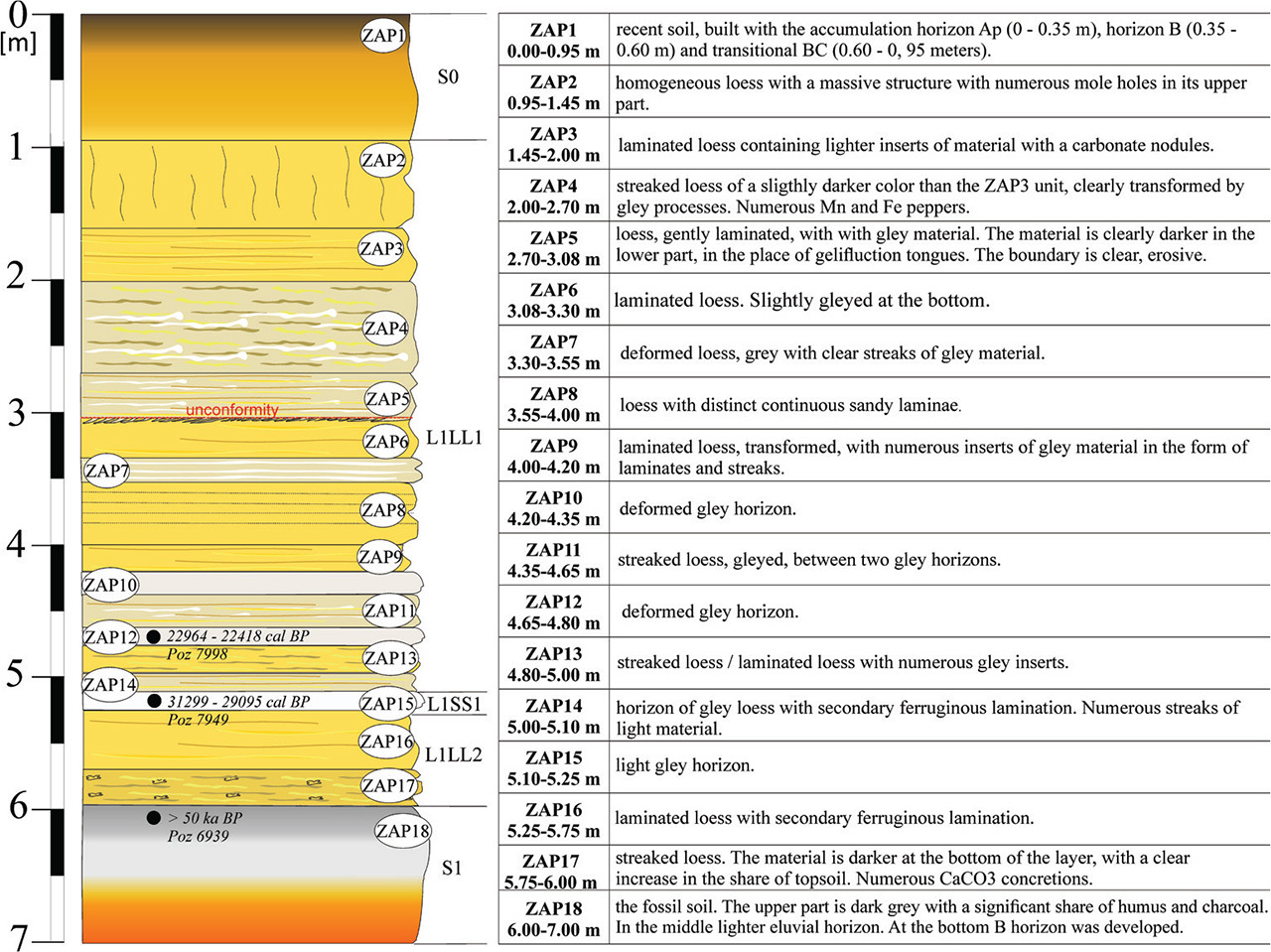
Characteristics of lithostratigraphic units and interpretation of periglacial phenomena were presented by Jary (2007, 2009, 2010), Jary and Ciszek (2013), Jary et al. (2016) and Krawczyk et al. (2017). New results from the 14C AMS dating of the Zaprężyn LPS were published by Jary (2007) (Fig. 2). Charcoals taken from the humic horizon of the fossil forest soil (ZAP18) have been dated as >50 ka BP (Poz-6939), humic substances from older tundra-gley soil (ZAP15) has an age of 31,299–29,095 cal BP (Poz-7649) and the age of humic substances from younger tundra-gley soil (ZAP12) is in range of 22,964–22,418 cal BP (Poz-7998). Based on the lithological data and three 14C AMS ages, Jary et al. (2016) designated five lithopedostratigraphic units in Zaprężyn LPS: two loess units (L1LL1 and L1LL2) and three soil units (S0, S1 and L1SS1). The presence of an ice wedge and its decay have been correlated with Upper Plenivistulian (MIS 2).
Fig 2.
Pedosedimentary sequence and description of the basic units in Zaprężyn LPS. Radiocarbon dating after Jary (2007). Stratigraphic interpretations after Jary et al. (2016) using labelling system after Marković et al. (2015).
For the younger part of the section, the issue of chronostratigraphic interpretation of the Zaprężyn LPS emerges. The 14C AMS ages are in conflict with the latest OSL results from the Bayreuth laboratory (Zöller et al., 2022). The ice wedge is thought to have developed in the Lower Plenivistulian (MIS 4) and melted at the beginning of the Middle Plenivistulian (MIS 3) according to the OSL ages from Bayreuth. In addition, Zöller et al. (2022) demonstrated the existence of an unconformity that most likely developed around 18 ka ago.
. Methods
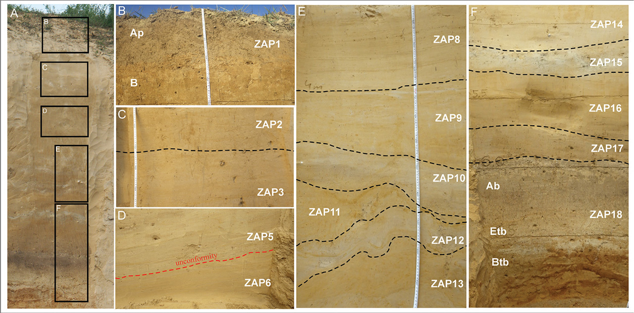
The field investigation included descriptions, rigorous cleaning of the profile and sampling for analysis. The profile was thoroughly cleaned to expose fresh material prior to description and sampling. The lithological description was then created (see Figs. 2 and 3). Antoine et al. (2009) presented continuous column sampling (CCS) used to collect samples for lithological investigations at 1 cm intervals. This technique relies on the careful cutting of continuous material to create a complete record of lithological variability and to eliminate gaps in the record.
Fig 3.
LPS from Zaprężyn: (A) – Whole Zaprężyn profile; (B) – modern soil; (C) – top of L1LL1 loess unit; (D) – unconformity; (E) – L1LL2 loess with deformed gley horizons; (F) – S1 soil and the bottom part of L1LL2 loess unit in Zaprężyn LPS.
. Lithological Analysis
Grain size distributions were determined by using a laser diffractometer Mastersizer 2000 in Soil Laboratory of Department of Physical Geography, University of Wrocław. H2O2 and 10% HCl were used to eliminate organic matter and carbonates before starting the measurement. Prior to measurement, sodium hexametaphosphate (Calgon) was added to the solution to facilitate greater dispersion.
Two granulometric indicators were employed here. As a metric for wind dynamics and atmospheric dust, the grain-size index (GSI) was derived using the formula GSI = (26–52 μm)/26 μm (Rousseau et al., 2007; Antoine et al., 2009). According to Vandenberghe and Nugteren (2001), the U-ratio index was derived as U-ratio = (16–44 μm)/(5.5–16 μm) to detect changes from low to high wind dynamics. The statistical parameters mean (Mz) and median (Md) were calculated too (Folk and Ward, 1957).
The Konica Minolta CM 600d spectrophotometer was used to determine the colour of the deposit. In this work, CIELab, the component units of the colour space are L* (luminance, or brightness [0–100]), a* (>0: red, 0< green) and b* (>0: yellow, 0< blue). The radiation reflected in this way is intercepted by a system with 36 detectors. The preparation process is the same as that provided by Gocke et al. (2014). The unique colour components L*, a* and b* are shown against RGB background colours (Sprafke, 2016). The fine-tuning of each RGB variable around its mean value, proportional to the distance between the maximum and minimum values from the profile mean, was carried out in two steps (RGB real, RGB k1) to facilitate the formation of the profile comprehensively. According to the method described by Sprafke et al. (2020), maximum tuning (RGB max) is accomplished by transforming RGB variables near their mean values to the entire range of this colour space (0–255).
. Luminescence Dating
Luminescence dating samples were extracted from distinct sections of the site, and carefully chosen for their representative characteristics. These samples were collected through a meticulous process that involved the use of clean vertical out-crops and thin-walled steel pipes. The Gliwice luminescence dating laboratory conducted the measurements as explained in the work by Moska et al. (2021).
Furthermore, advanced gamma spectrometry employing an HPGe detector from Canberra was employed to determine the dose rate. This method allowed the quantification of the uranium (U), thorium (Th) and potassium (K) content within the samples. The laboratory protocol outlined in Moska et al.‘s study (2021) guided this process. The dose rates were then computed utilising an online calculator for dose rates that integrates the latest conversion factors, as established by Tudyka et al. (2023). The assumed average water content stood at (15 ± 5)%, with all pertinent data for dose rate calculations comprehensively listed in Table 1.
Table 1.
Basic information about investigated samples.
For the measurement of OSL, quartz grains within the range of 45–63 μm were separated from sediment samples using standard treatments involving 20% hydrochloric acid (HCl) and 20% hydrogen peroxide (H2O2), as described in Aitken's work (1998). A density separation procedure, aided by sodium polytungstate solutions, was applied to isolate grains with densities ranging from 2.62 g/cm3 to 2.75 g/cm3. After sieving, the quartz grains underwent etching with concentrated hydrofluoric acid (HF).
Automated measurements for OSL were conducted using a Risø TL/OSL DA-20 reader equipped with a calibrated 90Sr/90Y beta source. This source delivered approximately 6.0 Gy/min to grains at the sample position. During OSL measurements, a 6 mm Hoya U-340 filter was utilised. The determination of equivalent doses was executed through the single-aliquot regenerative-dose (SAR) protocol, following the approach established by Murray and Wintle (2000).
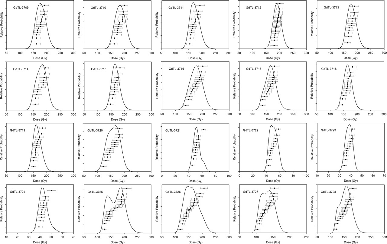
Final equivalent dose (De) values were derived for all samples using either the central age model (CAM) or the minimum age model (MAM), employing the ‘Luminescence’ R package developed by Kreutzer et al. in 2020. The dose distributions obtained were graphically represented in Fig. 4, illustrating relative probability density functions in accordance with Berger's framework (2010). Notably, all samples exhibited an overdispersion parameter significantly below 20%, and the distributions appeared unimodal. As a result, it was reasonable to infer that the tested material represented a collection of well-bleached quartz, as indicated in Moska et al.‘s work (2019a,b). Consequently, the CAM was deemed appropriate for the final calculations of equivalent doses.
Fig 4.
Relative probability density functions for equivalent dose distribution for all investigated OSL samples. Relative probability density functions according to Berger (2010).
. Radiocarbon Dating Procedure
Radiocarbon dates were obtained for gley horizons occurring in the lower part of the section. Since there were no charcoals, roughly 1 kg of material from each sample was used to extract the humic acid component in the lab. Since humic acids are not the ideal substance for 14C dating, it is essential to verify dates. The standard chemical pre-treatment based on the acid-alkali-acid (AAA) procedure was employed for radiocarbon dating. The samples are first washed in hot HCl, then they are washed in sodium hydroxide (NaOH), as part of the AAA pre-treatment. For the AMS technique, graphite targets were created. These procedures were carried out in the Gliwice 14C laboratory while the graphite targets were sent to an outside lab for analysis of the radiocarbon content. The 14C ages for all samples were calibrated with the OxCal program version 4.4 (Bronk Ramsey, 2009) and the calibration curve IntCal20 (Reimer et al. 2020) and the results are shown in Table 2.
Table 2.
14C ages of gley horizons in Zaprężyn LPS.
[i] The age was calibrated using OxCal program v4.4 (Bronk Ramsey, 2009) with calibration curve IntCal20 (Reimer et al., 2020).
. Results and Discussion
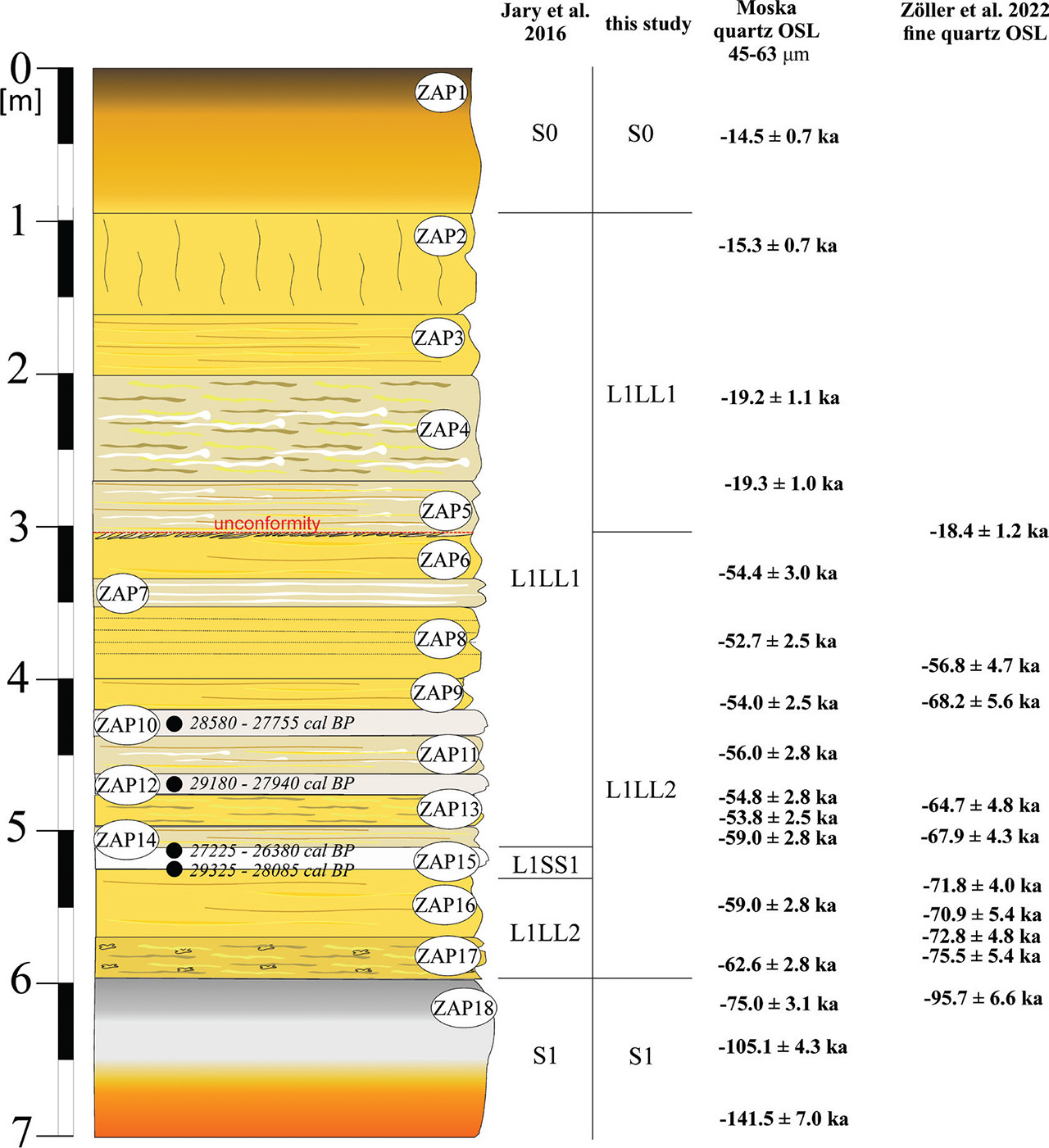
14C AMS ages earlier published by Jary (2007) are presented in Fig. 2. The new OSL ages for quartz (45–63 μm) and the 14C AMS ages are shown in Tables 1 and 2, respectively.
The new results of our research on the chronology of the Zaprężyn LPS confirmed the problem previously signalled by Zöller et al. (2022). All results of 14C ages obtained from humic acids in Zaprężyn LPS are underestimated, which is not a new experience in the study of 14C ages. Humic acids are always considered as a last-choice material for 14C dating. The 14C ages based on humic acids may be affected by the presence of humic acids from younger soil horizons located above a sample (e.g. Wild et al., 2013).
Due to parallel OSL dating performed in two independent laboratories, we believe that we are able to verify the previous stratigraphic interpretation of Zaprężyn LPS.
. Loess and Soil Units – Description and Interpretation
New stratigraphic interpretation is done based on the OSL ages obtained in two independent laboratories, field observations and the results of detailed granulometric studies (Fig. 4).
Zaprężyn LPS consists of four lithopedostratigraphic units (Figs. 5 and 6) developed during the Late Pleistocene and Holocene: two loess units (L1LL1, L1LL2) and two soil units (S0 and S1).
Fig 5.
Lithology, fraction percentages, grain-size parameters and stratigraphic units (acc. Marković et al. (2015) in the Zaprężyn LPS).
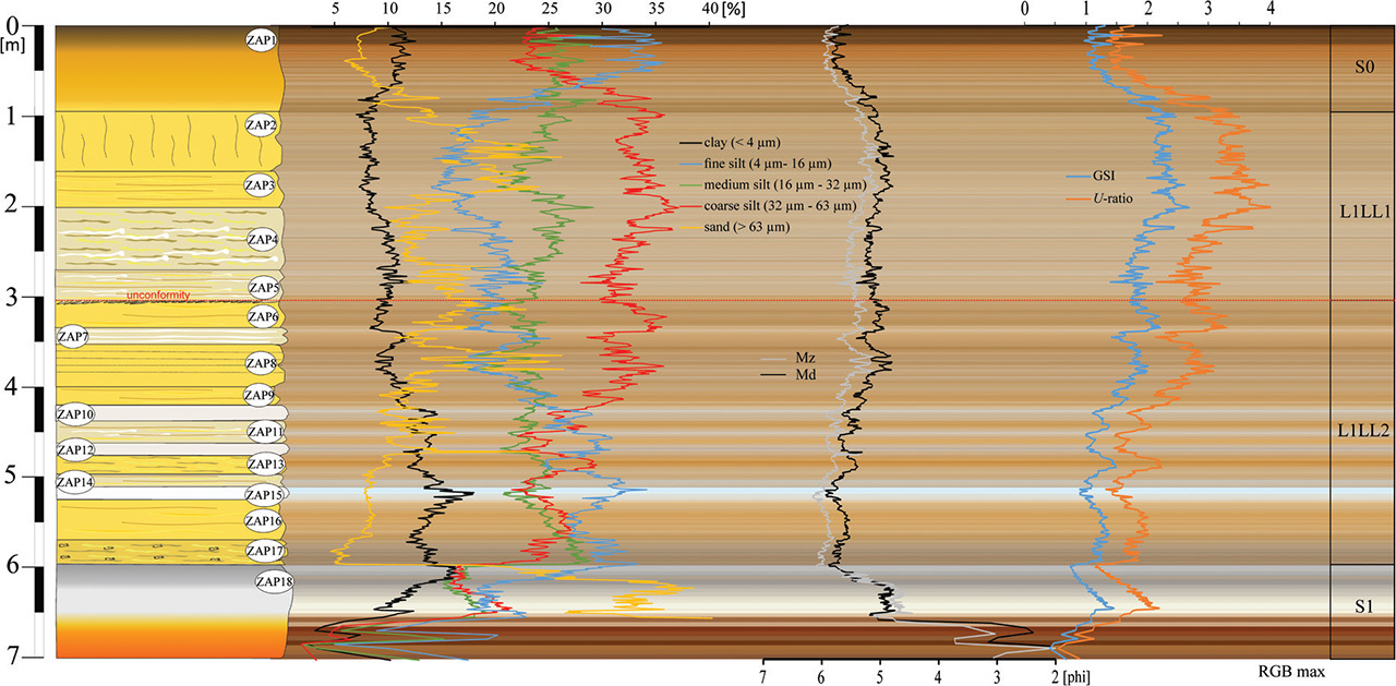
Fig 6.
The new 14C and OSL ages obtained in Gliwice laboratory, OSL ages published by Zöller et al. (2022) and revised stratigraphical interpretation of the Zaprężyn LPS.
. S1 soil unit
A fossil soil S1 was developed in the lowest part of the section (ZAP18). This luvisol is underlain by fluvioglacial Warta stage sand and gravel deposits, with illuviation clearly visible in the upper part. Due to the basic lithological characteristics of the substrate, the illuvial horizon Bt is not clearly defined. Both the accumulation A horizon and the eluvial horizon Et above have concentrations of charcoals that are just slightly distorted. Using 14C AMS, these charcoals were dated to be older than 50 ka BP (Fig. 2; Jary, 2007). According to the OSL dating data provided by Zöller et al. (2022) and Moska (this work) (Fig. 6), this unit is of Eemian-Early Vistulian age (MIS 5; Marks et al. 2016). All loess profiles in south-western Poland, S1 units, share comparable morphological characteristics. However, it clearly differs from the loess profiles in central and eastern Poland, where in the upper part of the S1 soil unit a thick chernozem has developed (Jersak, 1973a,b; Maruszczak, 1991; Jary, 2007; Jary and Ciszek, 2013).
. Loess unit L1LL2
L1LL2 loess unit occurs above the S1 soil unit (ZAP17-ZAP6). The Zaprężyn LPS L1LL2 unit is distinguished by its substantial thickness (3 m) and the presence of several different tundra-gley layers (ZAP15, ZAP12, ZAP10 and ZAP7). As in many other loess sections in SW Poland, the S1 and L1LL2 units' boundaries are clearly defined (Jary, 2007, 2010). A thin layer of loess/soil colluvium is present above this boundary (ZAP17). The L1LL2 unit is primarily composed of fine silt (4–16 μm) in the lower section and coarse silt (32–63 μm) with sand (>63 μm) inserts in the top part. The sharp, erosional barrier separates the L1LL2 loess from the unit above. Although the ages obtained in the Bayreuth laboratory by Zöller et al. (2022) are often a little older than in Gliwice, the OSL dating results of the two laboratories are comparable. With the help of the acquired data, the studied unit can be correlated to the Lower Plenivistulian (MIS 4). Numerous tundra-gley horizons found in the L1LL2 unit may be connected to the Lower Plenivistulian cyclic climate change. Similar characteristics have been observed in the Biały Kościół (Jary, 2007; Moska et al., 2015; Skurzyski et al., 2020); Złota (Jary, 2007; Moska et al., 2018; Zöller et al., 2022); and certain LPSs in Saxony (Meszner et al., 2011; Meszner and Faust, 2016).
. Ice wedge pseudomorph in L1LL2 unit
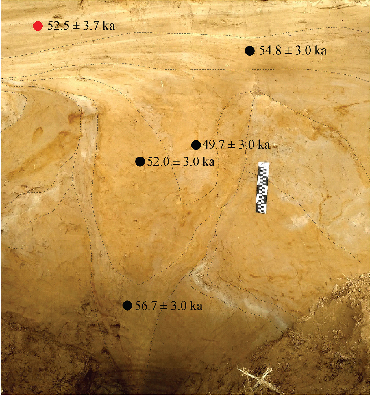
Zaprężyn LPS is the only loess site in south-western Poland where the ice wedge pseudomorph in the L1LL2 loess unit was observed. Ice wedge casts of this generation have not been discovered in any other loess region of south-western Poland, despite complete field exploration (Jersak, 1975, 1976, 1991; Jary 1996, 2007, 2009, 2010). The presence of the Lower Plenivistulian permafrost conditions in the Trzebnica Hills is confirmed by the ice wedge pseudomorph. The onset of the Middle Plenivistulian (MIS 3) is when the permafrost breakdown began, according to OSL ages (Fig. 7).
Fig 7.
Results of OSL dating of the ice wedge pseudomorph in Zaprężyn LPS: red dot - Zöller et al. (2022) result; black dots – Moska OSL results.
. Unconformity
The upper border of the L1LL2 loess unit (between ZAP6 and ZAP5) is erosive, as described earlier (Zöller et al., 2022). A loess unit L1LL1 is seen above. According to the results of OSL dating, this unconformity indicates a period of time that is >30 ka (Fig. 6). The absence of a L1SS1 soil unit, which was most likely entirely eroded here, is explained by this unconformity. The deposition of loess above the unconformity began 18–19 ka, just after the Last Glacial Maximum (Marks, 2012). The unconformity surface can be considered proof of extremely hard climatic conditions that existed during the Last Glacial Maximum, caused by proximity to the ice sheet margin (ca 70 km from Zaprężyn LPS).
. Loess unit L1LL1
The thickness of the loess unit L1LL1 (ZAP5-ZAP2) is roughly 2 m. It consists mainly of massive and laminated loess and the grain size is dominated by the course silt fraction (32–63 μm), with several sand inserts (>63 μm). They most likely provide proof that loess deposition in the Upper Plenivistulian occasionally involved periods of relatively brief transport and intense wind dynamics (Jary, 2007; Krawczyk et al., 2017). According to the OSL ages, the L1LL1 loess in the Zaprężyn LPS was deposited between 19 ka and 14 ka, which is a relatively short period (Fig. 6). The end of the loess deposition in Biały Kościół according to OSL ages, occurred between 18 ka BP and 19 ka BP (Moska et al., 2011, 2012, 2019a). This supports the theory that the loess deflation and deposition zones moved over a significant climatic gradient between the northern and southern parts of south-western Poland during the Last Glacial (Jary, 1996; Jary and Kida, 2000; Lehmkuhl et al., 2021).
. Soil unit S0
Modern brown soil S0 has been developed at the top of the L1LL1 loess unit (ZAP1). The accumulation horizon Ap (0.00–0.35 m), the B horizon (0.35–0.60 m) and the transitional horizon BC (0.60–0.95 m) make up this genetic horizon system. Due to its morphological position, the S0 soil is relatively thin and is located on a farmed, eroding slope surface. The soil substrate OSL age suggests that the material may have been deposited even during the Late Glacial of the Vistulian glaciation.
. Conclusions
In this study we present the obtained results of OSL and 14C AMS dating of the Zaprężyn LPS, the northernmost loess section in south-western Poland. We compared the studied LPS with other sequences, especially with the Biały Kościół LPS, pointing out the similarities and differences between corresponding stratigraphic units.
The most important conclusions are:
The results of LPS dating should be interpreted with caution.
All results of 14C ages obtained from humic acids in Zaprężyn LPS are underestimated.
Comparing the dating results from the two laboratories, the upper part of the profile showed that the dating results are in agreement. The data from the Gliwice laboratory are clearly younger in the lower part of the LPS, especially in L1LL2.
Zaprężyn LPS is composed of a relatively well-developed Lower Plenivistulian L1LL2 unit. The Upper Plenivistulian L1LL1 loess unit is represented only by the final phase of its deposition.
The ice wedge pseudomorph confirms the presence of permafrost conditions in this area during the Lower Pleniglacial. The permafrost decay occurred at the beginning of the Middle Pleniglacial.
The unconformity can be interpreted as a proof of extremely hard climatic conditions during the Last Glacial Maximum caused by proximity to the ice sheet margin.
The Zaprężyn LPS confirms the hypothesis about a considerable climatic gradient between the northern and southern parts of the study area which influenced on migration of the loess deflation and deposition zones during the Last Glacial.