
. Introduction
The current paper is addressed mainly to users of luminescence results obtained in the Gliwice Luminescence Laboratory (GLL) and other researchers who would like to set up their own laboratories. We describe procedures necessary for calibration of the measuring devices used in our laboratory. Technical details of such nature are not always easy to find in articles related to the presentation and interpretation of luminescence results themselves.
Currently, numerical dating using luminescence methods is widely applied in geosciences and archaeology in establishing the ages of sediments and archaeological artefacts (Liritzis et al., 2013). There are many luminescence laboratories in the world, which produce thousands of results every year. For using the luminescence methods, it is crucial to ensure the quality of the luminescence results obtained. This includes applying appropriate measuring procedures, like the single-aliquot regenerative-dose (SAR) protocol (Murray and Wintle, 2000) and calibration of the measuring equipment using a high-quality calibration and reference materials. This may include standards supplied by the International Atomic Energy Agency (IAEA) for gamma spectrometry or calibration quartz (e.g. supplied by Risø, Hansen et al., 2015) for calibrating the internal beta sources installed in the luminescence readers. Problems with the calibration of measuring equipment only come to light in the course of measurements in laboratory intercomparisons. The last large-scale intercomparison to determine the degree of coherence of luminescence dating measurements made by different laboratories was undertaken between 2006 and 2012 by 30 different laboratories and was coordinated by the Nordic Laboratory for Luminescence Dating. The obtained results were published by Murray et al. (2015) and showed how much still needs to be done to standardise the measurement procedures as a basis for obtaining comparable results.
We hope that the set of relevant measurement procedures, as well as the reference materials used by the GLL, presented in this manuscript can be an example of a reliable approach to ensuring the quality of the luminescence ages of tested materials.
Currently, the GLL is one of two laboratories working in Poland (the second one is in Toruń). Historically, luminescence dating has been applied in Poland for approximately 40 years, primarily for quaternary research, and was first implemented by M. Prószyński at Warsaw University, J. Butrym at Lublin University, S. Fedorowicz at Gdańsk University and M. Pazdur and A. Bluszcz at the Silesian University of Technology in Gliwice. The first studies addressing key aspects related to using luminescence phenomena for dating were published in Poland in the 1980s (Fedorowicz and Olszak, 1985; Bluszcz, 1986a, 1986b; Pazdur and Bluszcz, 1987a, 1987b). Currently, the laboratory is equipped with four optically stimulated luminescence dating (OSL/TL) readers (two Daybreak and two Risø), three high-resolution gamma spectrometers and three μDose systems (Tudyka et al., 2018).
. Methods
Establishing the luminescence age of a geological deposit requires different types of measurements. At this point, it is necessary to illustrate which laboratory measurements and procedures are vital to obtaining a single result of dating and how it can be interpreted. As a part of scientific services, the GLL focuses on quartz dating for all fractions using the standard SAR protocol (Murray and Wintle, 2000). Therefore, the following description is not relevant to feldspar dating.
Starting from the simplest definition, only two parameters are needed to determine the age of the sample to be tested: Age = De/Dr, where De is the equivalent dose determined using a luminescence reader, and Dr is the dose rate most determined using radiometric or analytical methods. The research aimed at improving the precision and accuracy of both values is carried out continuously, i.e. to improve the quality of the values of De (e.g. Anechitei-Ducu et al., 2018) and Dr (e.g. Kessler et al., 2018; Tudyka et al., 2020).
. Sampling
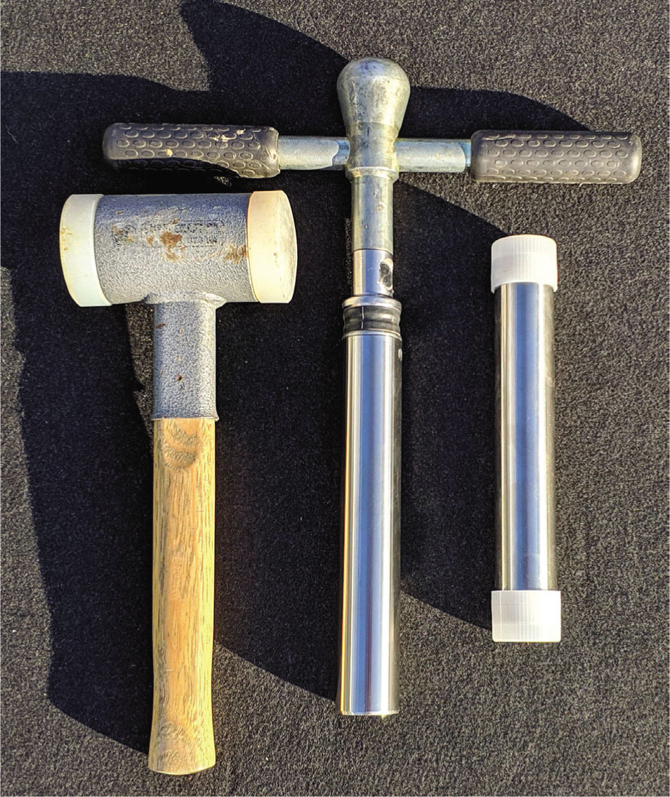
One of the most important aspects of luminescence dating is the appropriate selection of places from which the research material is collected. The elimination of undesirable uncertainties begins with the correct and appropriate sampling (Moska, 2019). The GLL uses the Eijkelkamp system (Eijkelkamp Soil & Water factory; Fig. 1), which meets all the requirements needed for the collection of samples for luminescence dating, including the ease of use, combined with the possibility of collecting material from even very hard sediments, and total protection of the collected material from sunlight. The Eijkelkamp system's design and the materials used to ensure safe and comfortable sampling conditions. This is particularly true about the protection of the collected material from sunlight, which is crucial for the OSL method.
Using metal pipes for collecting material from locations like walls or foundations of ancient buildings is not practicable. In such cases, a cordless drill with a coring saw (Fig. 2) is used to collect cores with a length and diameter of up to several centimetres.

. Dose rate determination procedure
The determination of the dose rate is an integral part of luminescence dating, and the precision and final quality of the luminescence dating strongly depend on the precision and accuracy of the dose rate determination. The ionising radiation to which minerals in the sediment are subjected originates from the 238U, 235U and 232Th decay chains and the isotopes 40K and 87Rb, which are natural components of the Earth's crust; in addition, there are secondary cosmic rays. At present, several methods are used for determining the concentration of the listed radioisotopes to assess dose rate in luminescence laboratories worldwide (Cunningham et al., 2018; Sjostrand and Prescott, 2002; Sanderson, 1988).
In the GLL, three radiometric methods are used for determining 238U, 232Th decay chains and 40K content, namely, high-resolution gamma spectrometry, portable gamma scintillation spectrometry and the μDose system.
In the case of typical geological materials, one may safely assume the availability of several hundred grams of raw material for laboratory research purposes, and high-resolution gamma spectrometry can be an option. However, with regard to archaeologically significant material or sediment cores, a large amount of material is rarely available, and only a small piece of ceramics or a few grams of the cored material may be available for testing. In such cases, the μDose system measurement can be preferred as <3 g of material is needed. An additional problem with testing archaeological samples is possibly a significant difference in the content of natural radioisotopes in the samples themselves in comparison to the surrounding sediment. This can be, for example, assessed using portable gamma scintillation spectrometry. The Laboratory, therefore, always asks for additional samples of surrounding sediment in the case of dating archaeological artefacts as well as for geological, geographical and geometrical descriptions.
Depending on the material type, the most suitable dose rate measurement procedure is selected. In general, the dose rate is modelled considering the best available knowledge and estimates with:
where ΣDi is the sum of all known α, β, γ and cosmic dose rate contributions. In most cases, dose rate conversion factors are applied after Cresswell et al. (2018). If applicable, alpha efficiency correction is used (Rees-Jones, 1995). The grain size distribution is taken into account as described by Bell (1979) and Brennan et al. (1991), while chemical etching after Brennan et al. (1991) and Guérin et al. (2012). Water content correction is done as described by Aitken (1985) and Aitken and Xie (1990). Specific geometry, depth and geographical location are also included if appropriate (Moska et al., 2018b or Chruścińska et al., 2014). More detailed information on how those dose rate corrections are applied can be found, for example, in Durcan et al. (2015).. Gamma spectrometry
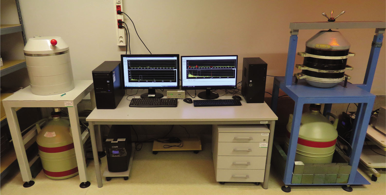
In the GLL, routinely high-resolution gamma spectrometry is used to determine the dose rate, which is calculated from radioisotope specific activities. GLL is equipped with three high-resolution gamma spectrometers (Fig. 3). Two of them are equipped with extended-range germanium detectors. In one case, the germanium detector is characterised mathematically and equipped with the LabSOCS Software (CANBERRA). The gamma spectrometers are additionally used for measurements of the activity of various isotopes for environmental and technical studies (Poręba and Bluszcz, 2007; Tylman et al., 2013; Poręba et al., 2019a). The laboratory participated several times in comparative measurements, including the measurements organised by the Nordic Laboratory for Luminescence Dating Centre in Risoe (Murray et al., 2015). Development work at the GLL led to the design of a new measurement container for gamma spectrometry, the gBEAKER which prevents radon loss from the measured sample (Poręba et al., 2020).
Fig 3
High-purity Germanium (HPGe) gamma-ray spectrometers in the GLL. GLL, Gliwice Luminescence Laboratory.
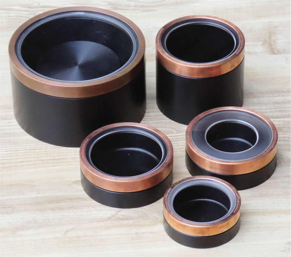
For a typical geological sample, the material is dried and then crushed in a designated room. Next, samples are stored for at least 21 days in the gBEAKERs where >98% of 222Rn emanating from the sample remains in the container (Poręba et al., 2020). This ensures that the 222Rn daughters can reach equilibrium with 226Ra. The size of the container depends on the amount of sample (Fig. 4). The mass of investigated samples is usually in the range between 50 g and 600 g.
Fig 4
The new type of containers (gBEAKERs) for samples used in High-Resolution Gamma Spectrometry (HRGS) was developed in GLL (Poręba et al., 2020). GLL, Gliwice Luminescence Laboratory.
To analyse radioactivity in samples, the gamma spectrometer must be calibrated. There are a few methods to achieve this. The two main methods are either through obtaining the total efficiency curve or through the measurement of standards prepared in the same geometry and matrix composition as the investigated samples (Murray et al., 1987). In the GLL, we prefer direct calibration for routine measurement for dose rate determination. To calibrate the gamma spectrometers as well as for quality control, reference materials provided by the IAEA are used: IAEA-RGU-1, IAEA-RGTh-1, IAEA-RGK-1, IAEA-375, IAEA-385, IAEA-444, Soil-6, as well as standards provided by the Polish National Radioisotope Institute (CLOR) or Eurostandard. For a standard sample designed for dose rate determination, the activities of radionuclides are determined using the lines shown in Table 1.
Table 1
Gamma spectrum lines used to determine the activities of the respective isotopes.
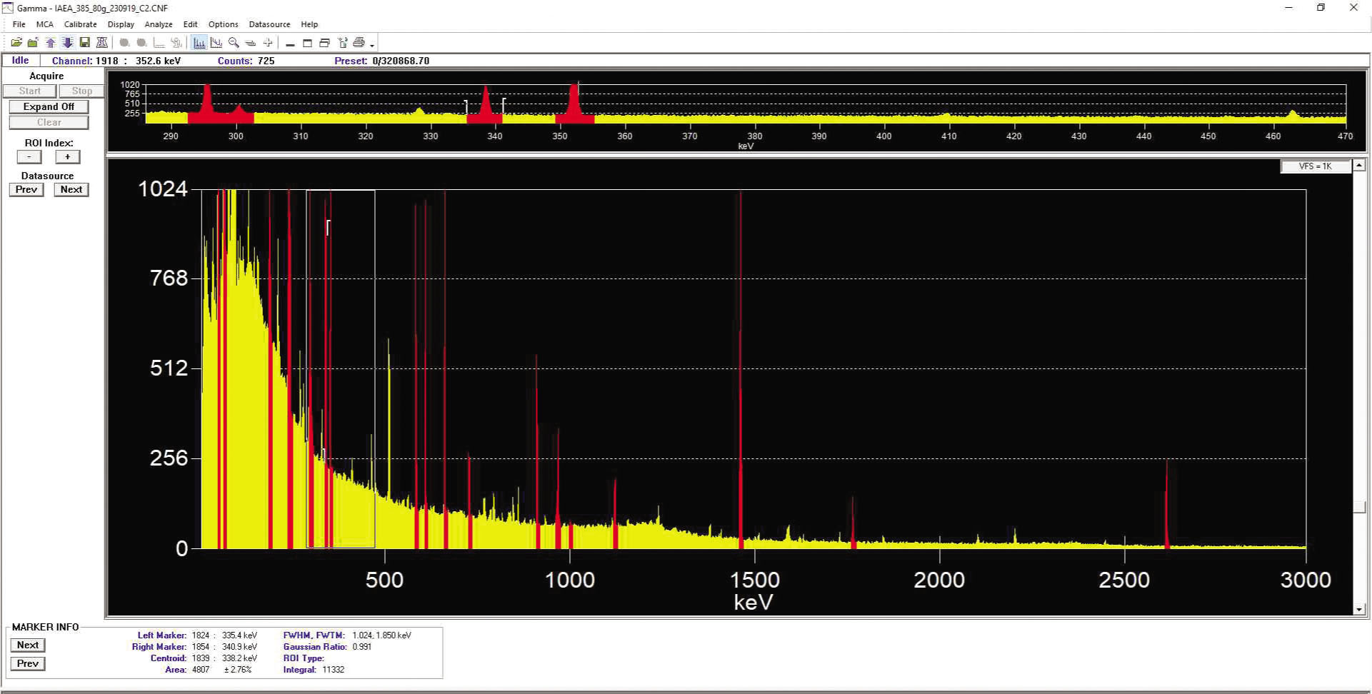
An example of a gamma-ray spectrum obtained for soil samples is presented in Fig. 5. In the case of low gamma radiation energy, to obtain the correct value of activity in the sample, self-absorption is included in the sample according to Cutshall et al. (1983). A background measurement is regularly performed to check background stability. The gamma room is ventilated using a computer-controlled system and air-conditioned to ensure stable operating conditions.
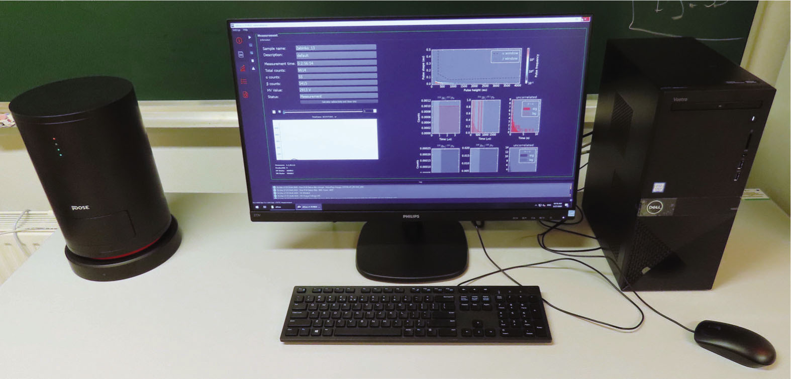
. The μDose system
A wide group of samples are beyond the capabilities of conventional gamma spectrometry. This includes but is not limited to: very small archaeological samples, samples where secular equilibrium in decay chains is questionable or internal alpha- and beta-dose rates (Jacobs, 2004; Jacobs et al., 2006) might contribute significantly to the final dose rate. For such samples, the μDose system (Tudyka et al., 2018; Fig. 6) is used. The μDose system detects alpha and beta particles along with four decay pairs that arise from the decay chains. In 2018, the GLL commissioned this system which combines the advantages of α (Aitken, 1985) and β (Bøtter-Jensen and Mejdah, 1988; Sanderson, 1988) counting measurement techniques with additional radioactive identification capabilities. The device allows for the measurement of small samples and verification of results as an independent method. The system electronically records α and β particles and their arrival times separately. This allows the detection of β/α and α/α decay pairs arising from 220Rn/216Po, 219Rn/215Po, 212Bi/212Po and 214Bi/214Po pairs, respectively. All decay pairs count rates and α and β particles count rates are used in assessing 238U, 235U and 232Th decay chains that are assumed to be in secular equilibrium. The β residual count rate is used to assess 40K radioactivity.
The μDose system is calibrated with the materials as described in Section 2.2.1. Besides, a reference material mix of IAEA-RGU-1, IAEA-RGTh-1 and IAEA-RGK-1 in proportion 1:1:1 allows improving the calibration. Dose rate and its uncertainties are calculated using Monte Carlo and Bayesian methods that are built in the μDose software and take into account correlations (Tudyka et al., 2020) allowing to obtain increased dose rate precision similar to high-resolution gamma spectrometry.
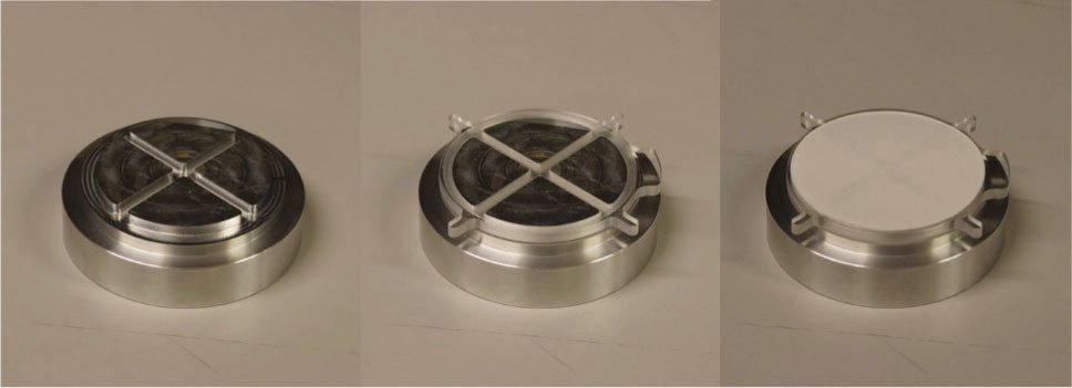
The μDose system requires different sample preparation than the HPGe detectors. First, the material must be dried. Then, 5–20 g of sample is ground down to particles of a diameter of approximately 20 microns using a planetary ball mill. This size is achieved in approximately 45 min at 200 rounds/min. Next, the sample must be placed on the 70 mm diameter sample holder, as shown in Fig. 7. Using a precise balance, exactly 3 g of the dried and ground sample is placed in the holder.
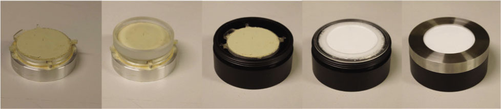
Next, the sample is placed inside the scintillation head, as shown in Fig. 8. Special attention should be paid to flattening the sample uniformly. The system calibration is only valid for the same mass of samples and standards.
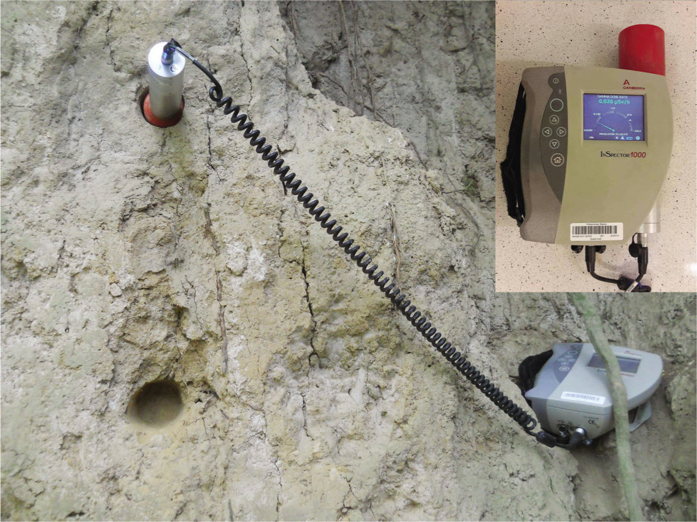
. Portable gamma spectrometer
The GLL is equipped with a portable gamma scintillation spectrometer manufactured by Canberra (InSpector 1000; Fig. 9) for recording energy spectra of ionising radiation in field conditions at sampling points for OSL dating. The portable gamma spectrometer was calibrated using concrete calibration blocks located at Oxford University (Rhodes and Schwenninger, 2007). Usually, four calibration blocks are used. Three of them are enriched with U, Th and K, and the fourth is pure concrete for background measurement. The portable gamma spectrometer is very useful for dose rate measurements, in particular, in areas where luminescence samples were taken from places close to boundaries between various sedimentation structures (which sometimes show a significantly different concentration of natural isotopes in the material – the best examples are sandy inserts in loess areas).
. Cosmic dose rate component
In addition to the measurement in the spectrometer, it is necessary to determine the dose derived from cosmic rays, which is calculated using the equation proposed by Prescott and Hutton (1994).
. Water content estimation
Water content is one of the basic parameters necessary for the correct determination of the dose rate. It has to be borne in mind that it is not, in this case, the current water content of the sediment, but a value that is representative for the entire deposition period. Based on the experience of the Gliwice luminescence dating laboratory, we approach this subject as follows:
- In the laboratory, the current water content and full saturation level are measured for all sediments.
- Usually, there is no possibility to precisely estimate sediment changes of water content for the last several thousand years (we can only make some approximations).
- Based on the collected environmental information for each position and hydrological condition, we determine the most likely humidity range for a given place.
. Equivalent dose measurement procedure
. Chemical pre-treatment
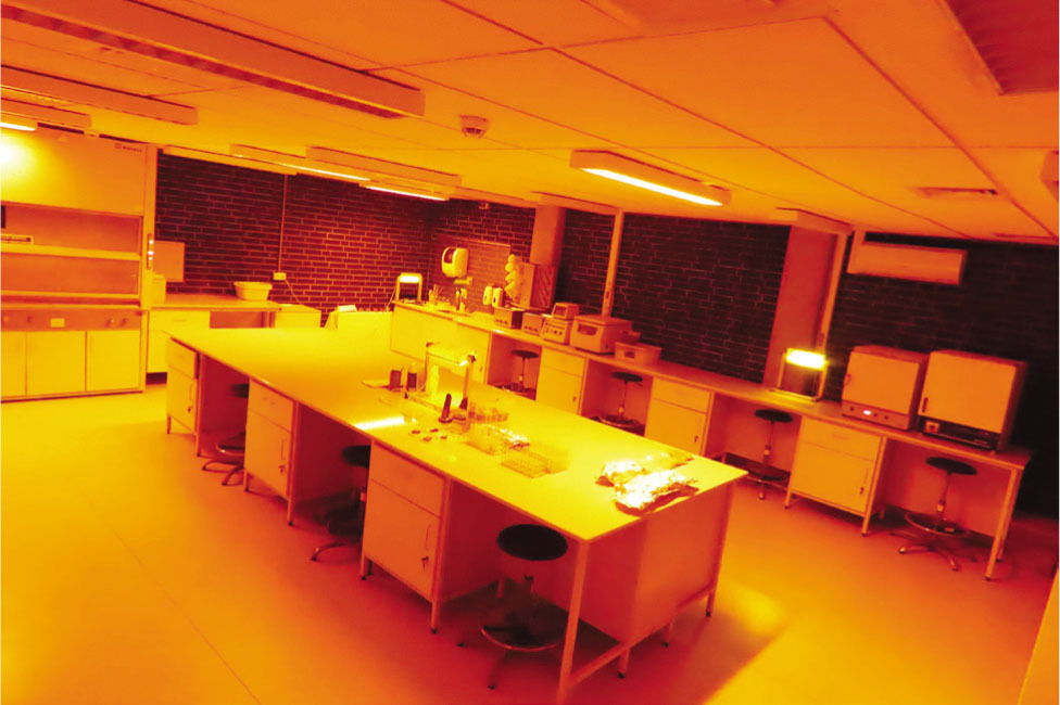
The entire procedure for preparing the material for OSL measurements takes place in a specialised chemical laboratory, where the only red light is used which does not remove the natural luminescence signal from the sample. The GLL's chemical preparation room is presented in Fig. 10. Throughout the entire laboratory, safe (deep golden amber) light is used. For this purpose, standard white fluorescent lamps equipped with an appropriate optical filter (professional certified foil – LEE filters 106 Primary Red) were used.
Chemical treatment is necessary to determine the equivalent dose from the extracted pure quartz. This procedure also depends on the size of the grains. Bigger grains (fraction above 45 μm up to 250 μm) at the beginning are treated with hydrochloric acid (20%) to remove carbonates, and hydrogen peroxide (20%) to remove organic matter. Between each step of the chemical preparation, the sample is rinsed with deionised water. A vital step in the extraction of pure quartz separation is the density separation using sodium polytungstate. During this procedure, a material with a density between 2.62 g/cm3 and 2.75 g/cm3 is separated. The used heavy liquid is collected, filtered and recycled.
The final step is treatment with concentrated (40%) hydrofluoric acid for 1 h to remove the outer layer of the grains of the quartz (about 10 μm) responsible for the absorption of alpha radiation dose (Aitken, 1985, 1998) and other minerals that might be still present after the density separation. After etching, to remove any residues, a final treatment with 20% hydrochloric acid for 20 min is used. For luminescence measurement, quartz extracted in this way is placed on steel disks with a diameter of 1 cm. Silicon oil (silkospray) as an adhesive is applied through a mask, and the grains are deposited as 6 mm circles.
The procedure for preparing fine grains (4–11 μm) is a little more complicated. The first step is to obtain the fraction below 45 μm using sieves. Next, as mentioned above, the material is treated with hydrochloric acid and hydrogen peroxide. Finally, the material is etched in concentrated hydrofluorosilicic acid (34%, H2SiF6) for a few days. Next, grains are washed minimum five times in distilled water, and hydrochloric acid (20%) is added for 2 h. After the following washes and drying, grains are ready for gravitational separation. The sample is placed in a tall test tube with acetone, in which gravitational separation of various fractions occurs over time. This procedure is repeated at least four times to obtain the most accurate material of the desired fraction. After obtaining the appropriate fraction, it is placed in 50 ml of acetone, and the well-mixed solution is then pipetted into 2 ml flat-bottomed tubes. Each tube, before filling, is fitted with an appropriately sized steel disc, on which, after the evaporation of the acetone, the fine grain fraction will be deposited. It is only then that the disks are ready for luminescence measurements.
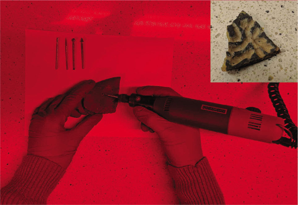
A similar procedure is necessary to extract quartz from the archaeological artefacts such as ceramics. First, a mini drill with milling cutters is necessary to extract material from the sample (Fig. 11). The outer layer of about 1 mm is sanded off, and the powder is collected from under this layer. The next steps are similar to the procedure, which is associated with the preparation of fine grains.
The most representative fractions for different kinds of sample material can be divided into three main ranges:
. Luminescence measurements
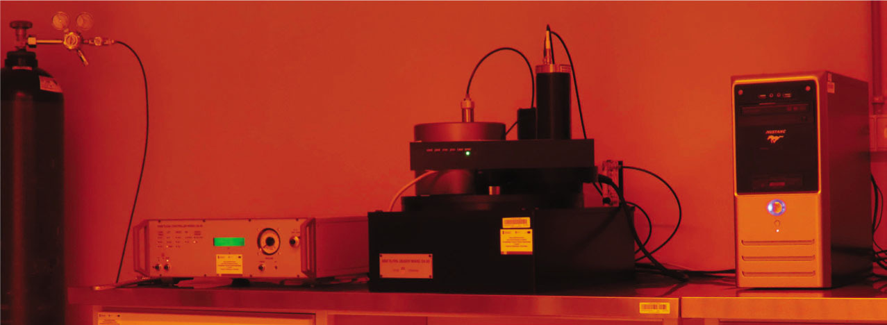
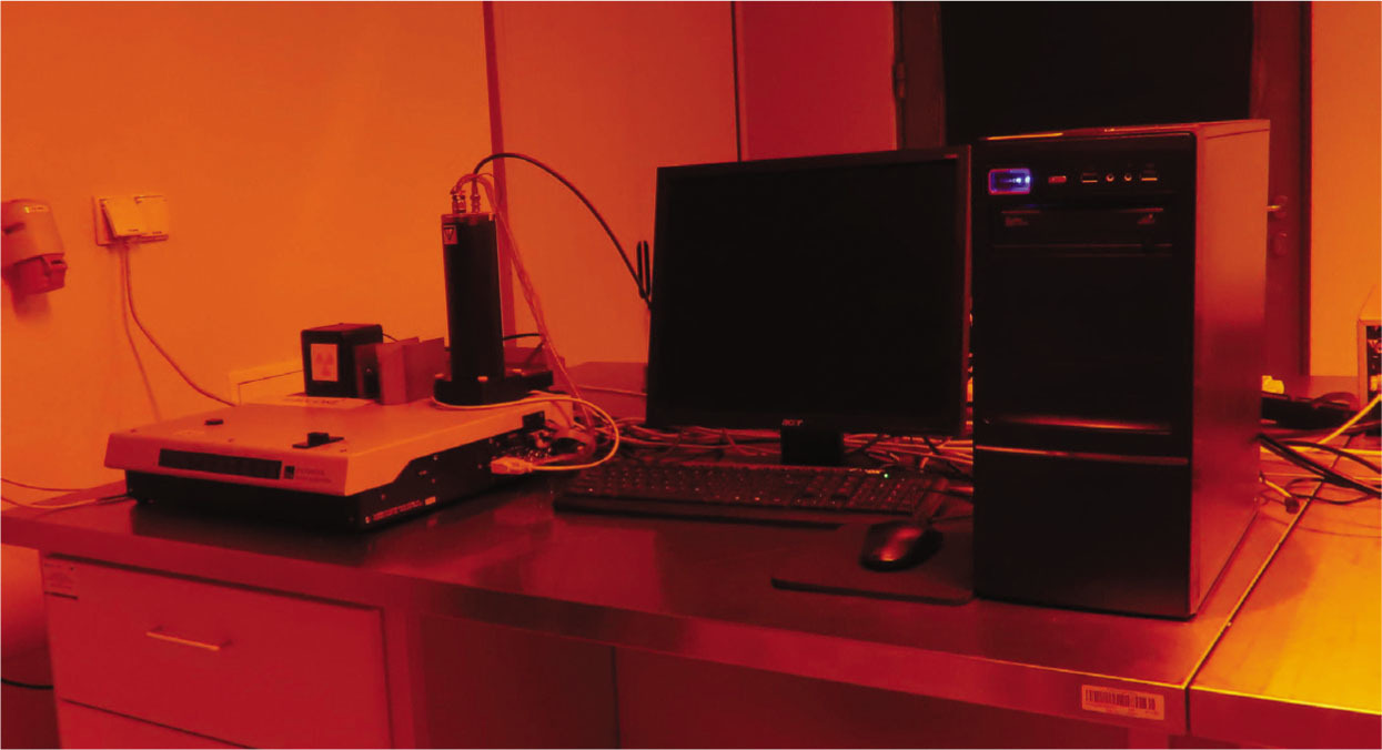
The GLL is equipped with four luminescence readers, two Risø TL/OSL DA-20 (Fig. 12) and two Daybreak 2200 TL/OSL automatic luminescence readers (Fig. 13), all readers are equipped with a calibrated 90Sr/90Y beta source. For calibration, in GLL, we use Riso quartz (Hansen et al., 2015). Readers also have two independent optical filters set depending on whether blue (green) or IR LEDs are used, 6 mm Hoya U-340 filter is usually used for the OSL detection (blue, green) and the BG39 (Schott)/CN7-59 (Corning)/GG420 (Schott) filter set are using for IRSL measurements.
. Luminescence procedures and De (equivalent dose) calculation
For quartz samples, equivalent doses are determined using the SAR protocol (Murray and Wintle, 2000). The readers are fitted with appropriate optical filters enabling the correct detection of the luminescence signal emitted from the tested samples. Table 2 presents all the necessary steps of the measurement process.
Table 2
Steps used in the protocol used for determining equivalent doses. For the quartz fraction, the SAR protocol (Murray and Wintle, 2000) is used.
In our laboratory, we focus on single aliquot measurements because single grain measurements are much more time-consuming and the final results do not necessarily deliver more information and precision (Thomsen et al., 2016).
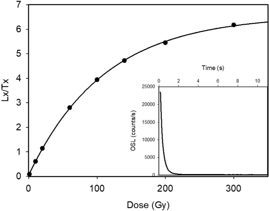
The result of the registration of natural luminescence for the sample and luminescence obtained following irradiation with specific regeneration doses is the so-called growth curve, an example of which is shown in Fig. 14 (a typical luminescence decay curve is shown in addition to the growth curve). This curve is created by fitting the appropriate function (usually saturating exponential) to the measurement points. The final result of the analysis of each growth curve is the determination of the equivalent dose.
Fig 14
The growth curve as a result of applying the SAR procedure for one quartz portion (the luminescence decay curve is shown below the growth curve). SAR, single-aliquot regenerative-dose.
In the SAR protocol, sensitivity changes that may occur from one measurement cycle to another are measured by the OSL response to a small test dose (Murray and Wintle, 2000). The corrected OSL ratio (regenerated OSL response/OSL response to the fixed test dose) should be independent of prior dose or thermal treatment. This is tested by repeating a particular regenerative dose after various larger values have been used and comparing the ratio of the two regenerated sensitivity-corrected OSL responses (known as a recycling ratio); this ratio should ideally be close to unity from 0.90 to 1.10 (Murray and Wintle, 2000). Preheating the sample can also cause the recuperation of the OSL signal (Aitken, 1985). To test this, a 0 Gy regenerative dose step is incorporated into the SAR protocol (Murray and Wintle, 2000). The luminescence signal should then be zero (this is known as the ‘recuperated’ luminescence signal). Any grains for which this sensitivity-corrected recuperated signal is >5% of the corresponding natural signal are rejected (Murray and Olley, 2002).
The dose recovery test is a basic requirement to determine the suitability of the SAR protocol. This is performed by administering a known dose in the laboratory and estimating it by the same measurement procedure as for dose estimates (Wallinga et al., 2000). During the dose recovery test, first, the natural signal is optically erased, and then a known dose is delivered to the sample. If the protocol works correctly, the ratio between the measured and the given dose should be in the range of 0.90–1.10.
For each analysed sample, measurements are usually performed for approximately a dozen individual quartz aliquots leading to obtaining a dozen ages. To determine the final value of the equivalent dose, an appropriate statistical model needs to be implemented – in this case, the central age model (CAM, Galbraith et al., 1999) was used. The introduction of a clearly defined statistical model to the final analysis of the measurement results allows a comparison of the obtained results with other laboratories dealing with luminescence dating. Typical examples of the presentation of luminescence results are shown in Fig. 15.
Fig 15
Graph of the probability density distribution (Berger, 2010) for two different samples, as typical examples of the presentation of luminescence results. Fig 15a present typical unimodal distribution, Fig 15b is an example of distribution characterised by higher value of overdispersion parameter.
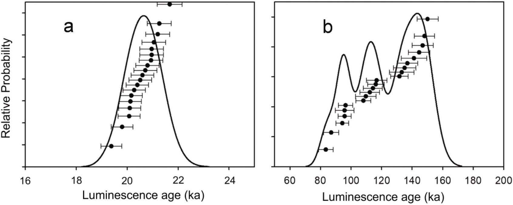
Within this model, the overdispersion parameter (σOD) is determined. This parameter refers to the distribution of the equivalent dose values for individual samples and increases with their dispersion. Fig. 15 shows two different examples of scattered values obtained for specific samples in the loess profile of Biały Kościół. These examples illustrate how different the results of individual quartz portions may appear in one sample. For the presented samples, the parameters of overdispersion were 5% and 19%, respectively. According to Galbraith's recommendations (Galbraith et al., 2005) for an overdispersion parameter <20% for the final equivalent dose determination, the CAM model should be used with one standard deviation (68% confidence interval) uncertainty. A group of adequately bleached samples (left graph in Fig. 15a) is characterised by lower overall overdispersion, typically about 10% or less (Arnold et al., 2007). Very often, we can meet distributions that have overdispersion parameters in the range between 10% and 20% (right graph in Fig. 15b). In those cases, usually, the typical unimodal shape of the distribution is not observed. It does not change the fact that CAM applied to all aliquots is still the most suitable model to estimate the final value of the De. Usually, fluvial samples can represent this group, and in this case, we can observe some asymmetry in the distribution (i.e. not statistically significant) (Arnold et al., 2007).
The sources of overdispersion are both intrinsic (e.g. counting statistics as described by Adamiec et al., 2012) and external (e.g. beta microdosimetry or incomplete bleaching; Duller, 2008). The effects of microdosimetry or bioturbation are likely to be reduced owing to the size of the aliquots. The most detailed analysis of stochastic modelling of the multi-grain equivalent dose was performed by Arnold and Roberts (2009), in which all possible number of sources of variation contributing to the commonly observed scatter in equivalent dose were examined.
It is vital not to interpret the multimodal distributions of the probability density, an example of which is the distribution on the right in Fig. 15b, as the possibility of the occurrence of three independent measurement results (there are three maxima of probability density) because this would over-interpret the obtained results and could lead to the falsification of the real age of the sediment. Another crucial piece of information is that we can read from such distributions the efficiency of resetting the luminescent signal in the sample during its redeposition. Fig. 15a shows a graph for a sample of material originating from a typical loess period L1LL1 (lower upper loess, Markovic et al., 2008), while Fig. 15b shows a sample from the soil complex S1. What follows, with a high degree of certainty, is that the sample derived from loess was much better and more evenly exposed to sunlight, allowing for a more precise zeroing of the signal from quartz grains. The sample from the soil will always be characterised by a significantly wider distribution because apart from the redeposition process, post-sedimentation processes such as bioturbation which is very distinct in well-developed soils, also play an important role.
. Application of results in projects
In its many years of cooperation with the scientific community in Poland and abroad, the GLL has participated in the implementation of a large number of domestic and five international grants. This level, scale and scope of involvement in the scientific research community is reflected in the quantity and quality of its proprietary publications and success in obtaining grants for leading scientific research.
We would like to mention at least the most interesting research projects implemented in our laboratory:
‘CONTINENT’ – aimed specifically at the high-resolution reconstruction of climatic conditions in the Holocene and Eemian periods. Several gravitational cores have been obtained from different locations on the lake to provide undisturbed sediment records covering the last ca. 150 ky. Different climate parameters were deduced from organic and inorganic components of the deposited matter. OSL was one of the methods selected for dating Lake Baikal sediments and the only capable of providing absolute dating for the Eemian period (Moska et al., 2008).
‘Establishing the chronology of loess formation in the eastern and western area of Poland based on high-resolution luminescence dating and geochemical studies of selected loess profiles’ – this project involves the use of a broad spectrum of research aimed at the reconstruction of climate change on the Polish territory over the past 100,000 years by a detailed analysis of the loess material. When we talk about climate change for the whole southern part of the Polish territory (because loess deposits occur only there), we have to remember that from the geographical location and the size of our country, the climate is not uniform. In the western part of Poland, there is a clear influence of the Atlantic climate, while in the east, continental climate, therefore considering the whole climate change in the past. In this project, a stratigraphic model was based on the detailed geochemical studies and a series of luminescence and radiocarbon dates (Moska and Bluszcz, 2013; Moska et al., 2011, 2012, 2013, 2015, 2017, 2018, 2019a, 2019b).
‘Settlement strategies, activity and natural environment of late Palaeolithic hunters and gatherers in the upland areas of Poland on the example of a complex of sites from Sowin’ – the project aimed at presenting a new chronological model of recolonisation of the area located north of the Sudetes and the Carpathians after Late Glacial Maximum (LGM). Until recently, it was believed that reoccupation of these areas occurred only due to the Magdalenian people. New chronometric data (radiocarbon and OSL) coming from the Magdalenian and Epigravettian sites together with the application of Bayesian modelling of new records allowed us to present another model. In light of the new research, it seems that the groups classified as the Epigravettian and Magdalenian could have coexisted at the same time in the same areas. The new model states that it is possible to assume the coexistence of these groups during 2300 years between 16,500 and 14,200 years BP (Wiśniewski et al., 2017).
‘The disappearance of the last ice sheet in the area of the South Baltic in the light of dating reservoir sediments and glaciofluvial deltas by the OSL method’ – the project was concentrating on detailed OSL dating of glaciofluvial and ice-marginal lake sediments which occur between end moraines of the Słupsk Bank and the Polish coast. As a result of research, it was found that the mode of deglaciation was changed from frontal and aerial into subaqueous after ice sheet retreat from moraines of the Gardno Phase. A large ice-marginal lake existed in front of the ice sheet during the Słupsk Bank Phase. The average age of this episode during the last SIS decay is 15.2 ka with a standard deviation of 0.9 ka (Uścinowicz et al., 2019).
‘Life and death of an extinct rhino (Stephanorhinus sp.) from western Poland in the light of interdisciplinary paleoenvironmental research’ – the sedimentary sequence has been the object of intense interdisciplinary study, which has resulted in the identification of at least two palaeolake horizons. Both yielded fossil remains of large mammals, alongside pollen and plant macrofossils. All these proxies have been used to reconstruct the environmental conditions prevailing at the time of deposition as well as to define the geological context and the biochronological position of the fauna (Sobczyk et al., 2020).
‘Palaeohydrological Extreme Events – evidence and archives’. Results from geomorphological, sedimentological and geochronological analyses, together with micropaleontological and mineralogical characteristics of lacustrine deposits in five locations within the Kuray intermountain depression, southeast Altai, mountains of south Siberia, support the thesis of repeated formations of ice-dammed lakes during MIS-2 and their draining by high energy floods. OSL was a tool to estimate the age for a sandy layer at the top of the diluvial (i.e. large flood) deposit, revealed in a sedimentary sequence of the 1570 m a.s.l. strandline – one of the lowest preserved strandlines in the western part of the basin (Agatova et al., 2020).
‘Multi-proxy investigations and advanced methods of determining numerical time scales in the reconstruction of the evolution of inland dunes in Poland during the end of the last glaciation’ – the European Sand Belt in Central Europe is a remarkably interesting remnant of the Late Glacial aeolian accumulation. Due to its geographical location, Poland is characterised by very extensive dune areas, which occur both in the form of large dune fields and individual dunes scattered throughout the country. Over the last several dozen years, a large volume of scientific and research works have been devoted to the stratigraphy of inland dunes. From the very beginning of the stratigraphic research, some researchers posed a purely hypothetical theory of the earlier formation of aeolian covers in the southern part of Poland (Older Dryas), and only later in the northern part (Younger Dryas). The assumptions of the hypothesis seem to be justified since the width of the European Sand Belt in Poland exceeds 400 km in the north-south direction. Such a significant spread should allow the detection of the temporal and spatial gradient of the formation of the aeolian units (Moska et al., 2020).
‘Correlation of primary loess profiles of Ukraine based on luminescence dates’ – project concerns the issues of age as well as lithological and pedological development of the loess-paleosol sequences selected after direct research at the Ukraine territory. For dozens of identical samples, a series of comparative laboratory TL dating (Gdansk, Lublin) and OSL dating (Gliwice) was performed, supplemented by the physicochemical and micromorphological analyses (Fedorowicz et al., 2013, 2018).
‘Reconstruction of anthropogenic soil erosion on selected loess areas of South Poland by dendrochronology, luminescence and isotopes (Cs-137, Pb-210) methods’. In this project, the SAR-OSL dating method was used to study Holocene water slope sediment simultaneously witch 137Cs and 210Pbex to measure modern soil erosion and sediment accumulation. Research carried out as part of this project clearly showed that loess accumulated loops in the Holocene are suitable for dating by the OSL method and showed why, despite the relatively short transport over the slope, good bleaching of the original luminescent signal is observed (Poręba et al., 2015, 2019a, 2019b).
‘μDose’ this project was aimed to commercialise innovative solutions for measuring dose rate. The developed system, with the same name, offers new possibilities of increasing dose rate precession and accuracy, measuring small samples including internal dose rate and obtaining reliable dose rate in samples where secular equilibrium is uncertain. A detailed description of the μDose system is given in Section 2.2.2 and by Miłosz et al. (2017), Tudyka et al. (2018) and Tudyka et al. (2020).
. Final remarks
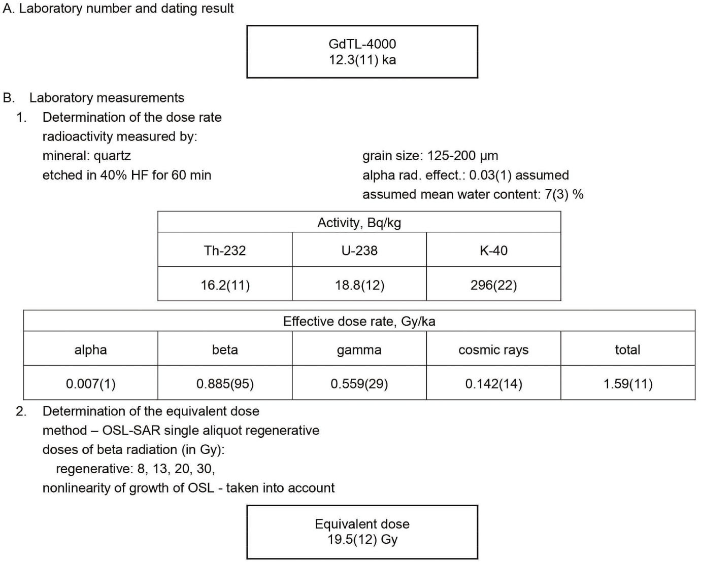
All final luminescence results are placed in the Laboratory's GdTL luminescence database, and a final report from luminescence dating is generated. A part of the report, all necessary information connected with a particular example is presented (see Fig. 16). Each dated sample has its unique laboratory number (e.g. GdTL-4000). The report also contains information about the fraction used for measurement, water content, the activity of 238U and 232Th decay chains and 40K, effective dose rates, the number of investigated aliquots and regenerative doses used in luminescence protocol. Finally, the equivalent dose and the age of the sample are presented.
The age limit of luminescence generally ranges from several years to hundreds of thousands of years. Among all dated samples in the history in the GLL, the youngest dated sample was colluvium loess from Szyszczyce (Poręba et al., 2013) with a result of 25 ± 8 years. Such young results are very difficult to obtain as the investigated material should have very good luminescence properties, as the lower age limit is severely restricted by the efficiency of signal resetting and signal sensitivity. On the other hand, obtaining very old results using OSL for quartz (a few hundred thousand years) is also very difficult and debatable because the upper age limit is controlled by the capacity of the crystal lattice to store electrons and the dose rate of the environment. The growth curve (see Fig. 14) usually begins to saturate at about 200 Gy, but this effect is fundamentally linked to the luminescence properties of the investigated material. This effect refers to the complete filling of traps such that continued exposure to emissions from radiation decay results in no more accumulation of electrons and thus no increase in luminescence signal. One should also be aware that the dose rate also depends on the natural concentration of natural radioisotopes in the tested material, and therefore its value varies greatly depending on the type. A very high value is characterised for bricks and ceramics (even >4–5 Gy per thousand years), for loess deposits this value oscillates around 3 Gy/ka and for sand dune <1 Gy/ka. The dose rate value determines the possibility of dating very old sediments, which is why in the GLL, the oldest samples were collected from a seaside cliff in Osłonino (Poland) for which the dose rate was extremely low (about 0.4 ÷ 0.5 Gy/ka), and this is why it was possible to obtain results for several of the samples at about 300 ka. Typically, luminescence ages show good agreement for samples of known age and ages derived from independent methods (Murray and Olley, 2002). The combined uncertainty in the measurement of De and the dose rate typically ranges from 5% to 10%, including random and systematic error.