
. Introduction
Long systematic instrumental records of climate data are rare and spatially limited (for a review see Jones and Bradley, 1992). Natural archives are therefore used to extract information about the climate in the past. Tree-rings are among the most commonly used proxy records, especially in temperate zones, where seasonal growth results in annually resolved tree-rings.
The standard methodology which is usually used to study the relationship between climate (e.g., temperature, precipitation, moisture, cloudiness etc.) and tree-ring proxies is to apply (multiple) linear regression (MLR; Cook and Kairiukstis, 1992). However, while linear transfer functions usually fit data well, there are some concerns about predictions for data points close to the edge of observed data and points out of the calibration data. Linear models assume that the dependency between tree-ring parameters and climate changes linearly from the most favourable to the most unfavourable conditions. This assumption is contradictory to the well-accepted concept of ecological amplitudes (Braak and Gremmen, 1987; Fritts, 1976), and trees can thus grow only in a limited range of growing conditions. The relationship between tree-ring parameters and environmental factors should, therefore, change when approaching the edges of ecological amplitudes.
There is growing evidence that nonlinear techniques are better at describing the relationship between tree-ring proxies and climate variables (Balybina, 2010; D'Odorico et al., 2000; Helama et al., 2009; Jevšenak and Levanič, 2016; Ni et al., 2002; Zhang et al., 2000). Sun et al. (2017) showed a significant improvement over linear regression by using linear spline regression and a likelihood-based model to explain nonlinearity in the relationship between tree rings and precipitation. One of the most accurate and tested process-based models, the Vaganov-Shaskin model (VS model, Shishov et al., 2016; Vaganov et al., 2011), uses a piecewise linear function to model the relationship between daily environmental data and tree-rings. A similar idea is implemented in a simplified version of the VS model – the VS-Lite model (Tolwinski-Ward et al., 2011). The advantages of using nonlinear models have also been demonstrated in other studies using tree-ring data, such as predicting resilience to disturbance (Billings et al., 2015), modelling tree growth response after partial cuttings (Montoro Girona et al., 2017) and predicting the response of tree growth to climate change (Williams et al., 2010).
In this article, we compare various regression methods. To this end, we used Vessel Lumen Area (VLA) tree-ring chronologies of pedunculate oak (Quercus robur L.) from two lowland sites in Slovenia. VLA is gaining importance in dendroclimatological studies, especially at mesic sites, where earlywood conduits often have a better climatic signal than traditional tree-ring width (Campelo et al., 2010; Fonti and Garcia-Gonzalez, 2008; Jevšenak and Levanič, 2015).
The formation of earlywood vessels usually starts at the end of March or early April (Goršić, 2013; Gričar, 2010), when the temperature or moisture threshold, i.e., the degree-day sum, is surpassed. This threshold is site-and species-specific. The period of most intense xylem cell production in oaks from nearby areas is April-May (Gričar, 2010), when the relationship between earlywood conduits and climate is more or less linear. Again, in the period from middle May-June onward, we expect saturation of the function that describes the relationship between earlywood vessels and climate. The two functions that could model such relationships more accurately (as compared to linear regression) are the sigmoid-shaped and piecewise linear functions. Both were applied in our study.
The goals of our study were 1) to analyse the relationship between VLA and climate, 2) to select predictors of VLA based on the results of the climate-growth relationship and 3) to apply those predictors to compare MLR and four different nonlinear modelling techniques (ANN, MT, BMT and RF).
. Material and methods
Study objects and wood-anatomical analysis
The two VLA chronologies used in our study were sampled from two lowland forest sites in Slovenia (Fig. 1). The selected sites are dominated by Quercus robur, but differ in some site-specific conditions (see Table 1). The two sites have approximately equal temperature distributions, while the QURO-2 site (meteorological station Ljubljana, Fig. 1C), gets slightly more precipitation than the QURO-1 site (meteorological station Maribor; Fig. 1D). Climate data for both meteorological stations were provided by the Slovenian Environment Agency (ARSO, 2017).
Fig. 1
A) Locations of the research sites (circles) and the meteorological stations (triangles), B) location of Slovenia in Europe and climagraphs of C) Ljubljana and D) Maribor. The lines of climagraphs represent mean monthly temperature and the blocks represent monthly amounts of precipitation.
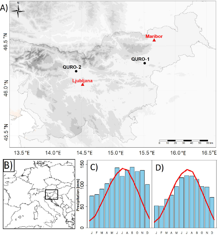
Table 1
General description of the analysed sites.
From each site, 6–8 mature and dominant trees (see Table 2, Fig. 2) were sampled for wood-anatomical analysis with a 10-mm increment borer. One core per tree was taken at breast height of 1.30 m. The extracted wooden cores were air dried, radially oriented and fitted in wooden holders. They were then sanded to a high polish in a laboratory, as suggested by Fonti et al. (2010). The sanding process starts with coarse 80-grit and ends with fine 1000-grit sanding paper. After sanding, vessels were filled with chalk, and high-quality images were taken with the ATRICS system (Levanič, 2007). ATRICS is an automated image acquisition system based on a motorised stage and a high-resolution microscope camera, which captures images and stitches them into a single, long image of the entire core. The captured images were analysed using the ImageJ program (Schindelin et al., 2012), combined with macro EWVA (Fig. 3; Jevšenak and Levanič, 2014). First, the contrast between the vessels and the adjacent surface was enhanced, based on the selected black and white threshold. Each group of vessels was then recognised as a consecutive year and, finally, vessel lumens were measured. In each tree-ring, all vessel lumens were measured, and the parameter vessel lumen area (VLA) was subsequently calculated, considering only vessels with an area greater than 10,000 μm2. The same threshold was used by Fonti and Garcia-Gonzalez (2008). VLA chronologies were not detrended, since we did not observe any age-related trend (see Fig. 4).
Fig. 2
Individual sample lengths. The shaded area represents the analysed period used for model comparison for QURO-1 and QURO-2.
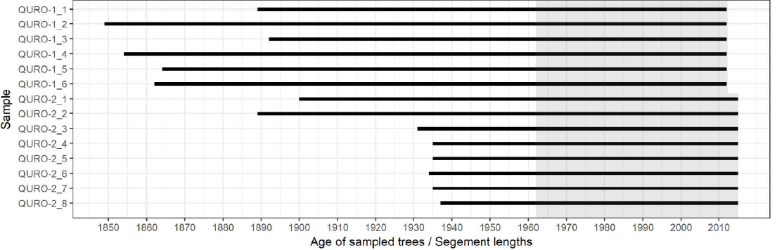
Fig. 3
An example of a workflow of earlywood vessel analysis with ImageJ and macro EWVA: A) original image, B) image converted to a black and white mask for segmentation of the original image, vessels below the threshold were excluded from the analysis, C) recognised groups of earlywood vessels belonging to different years overlaid over the original image and D) measured earlywood vessels.
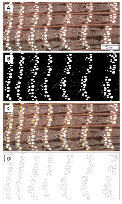
Fig. 4
Chronologies of vessel lumen area (VLA) for QURO-1 and QURO-2 with 95% confidence interval of the mean.
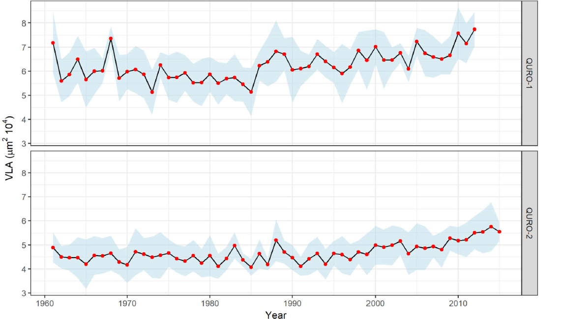
Table 2
Characteristics of site chronologies: number of samples (N), chronology span, mean and standard deviation (Std) of vessel areas, minimum and maximum range of vessel areas (Min – Max), rbar (r̄) and autocorrelation with lag 1, 2 and 3 (AC).
| Mean ± Std | Min – Max | |||||||
|---|---|---|---|---|---|---|---|---|
| Site | N | Chronology span | (μm2 104) | (μm2 104) | r̄ | AC_1 | AC_2 | AC_3 |
| QURO-1 | 6 | 2012–1961 | 6.259 ± 0.603 | 5.133–7.743 | 0.44 | 0.42 | 0.40 | 0.31 |
| QURO-2 | 8 | 2015–1961 | 4.691 ± 0.395 | 4.072–5.756 | 0.32 | 0.61 | 0.52 | 0.46 |
Nonlinear machine learning methods
The nonlinear methods used in our study belong to the field of machine learning. We used a single layer perceptron as an artificial neural network (ANN) (Bishop, 1995; Hastie et al., 2009), which we trained with the Bayesian regularization training algorithm (Burden and Winkler, 2008). The described ANN method is available in the brnn R package (Pérez-Rodríguez and Gianola, 2016; Pérez-Rodríguez et al., 2013) and usually fits a sigmoid-shaped transfer function.
Model trees (MT; Quinlan, 1992) are tree-structured models in which each terminal node in the tree contains a prediction in the form of a linear equation. A model tree is equivalent to a piecewise linear function and, when visualised, offers some interpretable features, such as the relative importance of predictors and the different linear equations used in the different terminal nodes.
In order to further improve the predictive capabilities of MT, bagged model trees (BMT) were used, which are derived by the ensemble method of bagging (Breiman, 1996). Bagging involves the construction of several bootstrap samples of data obtained through random sampling with a replacement, and learning an MT from each bootstrap sample. Combining the predictions of individual MTs in the ensemble prevents overfitting the data.
Random Forests (RF; Breiman, 2001; Ho, 1995) of regression trees is an ensemble method that applies a randomised regression tree construction algorithm to each of the bootstrap samples. In regression trees, the predictions in the terminal nodes are real value constants, rather than linear models. The randomised algorithm considers only a small number of randomly selected predictors at each step of tree construction. We used the MT, BMT and RF algorithms for learning from the RWeka R package (Hornik et al., 2009).
ANN, MT, BMT and RF are advanced algorithms used in the field of machine learning. These algorithms can also find linear relationships, in cases in which the dependency to be modelled is linear. We hypothesised that nonlinear techniques would provide better models,
which means more explained variance and lower error on validation data.
Modelling strategy and comparison of nonlinear methods for VLA prediction
Pearson correlation coefficients were used to analyse the climate-growth relationship between climate data and VLA chronologies to get a first impression of patterns in the climate signal. Secondly, based on the results of the climate-growth relationship, climate variables were selected to be used as predictors for VLA. MLR models were then fitted by using these predictors, and the statistical properties of these models were assessed. To fit MLR models, stepwise selection of predictors with backward elimination was used. In addition, model trees (MT) were fitted to explore the understandable rules for VLA predictions. Finally, the performance of linear and nonlinear machine learning regression methods was evaluated by 3-fold cross-validation (Witten et al., 2011), which is implemented in the compare_methods() function of the dendroTools R package (Jevšenak and Levanič, 2018).
In 3-fold cross-validation, the datasets were randomly split into 3 equal parts (folds) and models were systematically calibrated (learned) on 2 folds and validated on the remaining fold that had not been used for calibration (learning). To minimise coincidence due to specific train and test splits, cross-validation was repeated 100 times, and the mean and standard deviation of the performance metrics across all repeats of cross-validation were shown. To ensure objective comparison, the cross-validation splits were identical for all nonlinear and MLR models, which was achieved by using the set.seed() function in R (R Core Team, 2018).
In addition, for each individual cross-validation split, the different models were ranked in terms of the calculated performance metrics, with rank 1 representing the best performance. The ties.method argument from the rank() function in R was set to ‘min’. Both models with the same performance metrics values were therefore given the lowest rank. The sum of shares of rank 1 consequently does not necessarily equal 1. The mean ranks and shares of rank 1 for each method are reported in the Results section.
For each cross-validation split, MLR was fitted by a stepwise selection of predictors with backward elimination. For each individual MLR model, therefore, only statistically significant and non-correlated predictors were used. One of the major strengths of machine learning algorithms is that they can be run with a large set of predictors with no a priori assumptions regarding which predictors are most important, or the underlying nature of the relationship between the response and predictor variables. ML models were therefore trained using all available predictors.
In the preliminary experimentation phase, different parameter settings of the four nonlinear algorithms were explored. We optimised our methods by experimentation and with the caret R package (Kuhn et al., 2017). The train function from the caret R package sets up a grid of tuning parameter’s values for a number of regression routines, fits each model and calculates a resampling-based performance measure. The final models were tuned for each dataset separately and used to compare the performance of different regression algorithms. A list with tuned parameter values is presented in Supplementary Table S1.
The measures of performance used in our study were the correlation coefficient (r), the root mean squared error (RMSE; Willmott, 1981), the root relative squared error (RRSE; Witten et al., 2011), the index of agreement (d; Willmott, 1981), the reduction of error (RE; Fritts, 1976; Lorenz, 1956), the coefficient of efficiency (CE; Briffa et al., 1988) and the detrended efficiency (DE; Helama et al., 2018). Models with higher validation (testing) values of r, d, RE, CE and DE and lower values of RMSE and RRSE were considered to have better predictive capabilities. In addition, to address potential over- or under-prediction associated with a given approach, bias was calculated as the difference between observed and estimated mean response for the validation data. Bias is reported in the form of histograms for each method.
. Results
Chronology characteristics and the climate-growth relationship
The two site chronologies had a common increasing trend in VLA in the last 2–3 decades (Fig. 4). Even though the trees considered differed in terms of age (Table 1, Fig. 2) and were sampled from sites with different site characteristics, the increasing trend in VLA was obvious and consistent for both sites. The values of VLA in the QURO-1 chronologies ranged from 5.133–7.743 μm2104, while VLA values for QURO-2 ranged from 4.072–5.756 μm2104. Higher coherence between individual VLA chronologies was observed for QURO-1 (r̄= 0.44),while QURO-2 had less coherent individual chronologies (r̄= 0.32). Autocorrelation was significant in both analysed chronologies. On average, the vessels with the largest area were those from the QURO-1 site (Table 2).
VLA chronologies were compared to mean monthly temperatures and monthly sums of precipitation (Table 3). The two sites showed a very similar temperature pattern – VLA was significantly correlated with mean spring temperatures and mean temperatures from the previous growing season. Analysing only individual months of the current growing season, April had the strongest correlation coefficient at both sites. For the previous growing season, QURO-1 was correlated with temperatures from July to September, while QURO-2 correlated with temperatures from July to November. Only QURO-2 had significant correlations between the sum of precipitation and the VLA chronologies. Winter precipitation showed negative correlations with VLA from QURO-2.
Table 3
Pearson correlation coefficients between vessel lumen area (VLA) and climate data: mean monthly temperatures (TEMP) and sum of monthly precipitation (PREC) for QURO-1 and QURO-2. Months with capital letters refer to the current growing season, while months with lowercase letters refer to the year of the previous growing season. Only correlation coefficients with p ≤ 0.01 are shown.
Based on the correlation analysis, the predictors of VLA were selected for each site individually. All months with significant correlations from the previous growing season were averaged, so we obtained a single additional predictor representing the previous growing season temperatures. Precipitation values for the months from January to March were summed, so we obtained a single additional winter precipitation predictor for the QURO-1 site. All the monthly temperature variables from the current growing season with significant correlations were kept as individual predictors. The strongest linear relationship between VLA and monthly temperatures was observed for April, thus we expected to observe a more nonlinear relationship by adding temperature information for March and May. The final list of predictors for QURO-1 and QURO-2 is given in Table 4.
The predictors were fitted by the multiple regression method, using the stepwise selection of predictors (Table 5). None of the diagnostic plots of the linear regression models for the two sites showed any problematic patterns (see Fig. S1). As in the correlation analysis (Table 3), April temperatures were the most significant variables. Both models showed some similar patterns: 1) they excluded May temperatures as a significant predictor, 2) both models explained a similar amount of variance, 0.63 with QURO-1 and 0.62 with QURO-2 and 3) both models had a similar value for the coefficient for temperatures from the previous growing season.
For both sites, model trees (MT) were fitted to extract rules for predicting the VLA at each of the analysed sites (Fig. 5). For each instance (year), the values of its predictors determine which linear equation will be used to make the final prediction. For example, for QURO-1, if the mean April temperature (T_APR) is smaller than 9.97 °C, linear equation 1 (LM1) is used. Otherwise, the January-March sum of precipitation (P_JAN-MAR) is considered, with the threshold to select linear equation 2 (LM2) or 3 (LM3) set to 56.9 mm. This threshold indicates the point at which the relationship between VLA and the climate
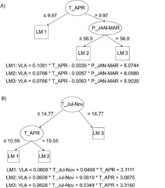
Table 4
Description of predictors of the VLA for QURO-1 and QURO-2.
Table 5
Multiple linear regression summary statistics for QURO-1 and QURO-2.
variables changes. While for QURO-1, T_APR is the most important predictor, for QURO-2 temperatures from the previous growing season (T_Jul-Nov) are in the root of MT. If T_Jul-Nov is greater than 14.77°C, linear equation 3 (LM3) is used; otherwise T_APR is considered. Finally, if T_APR is greater than 10.55 mm, MT will use LM1; otherwise LM2 is applied to make the final prediction.
Comparison of different ML algorithms for VLA prediction
MLR, ANN, MT, BMT and RF were used to model the relationship between VLA and the selected climate predictors (Table 4). The models were primarily evaluated in terms of their performance metrics on validation data (Table 6), which can be considered to be objective indicators. For QURO-1, ANN provided the best performance in 53% of individual cross-validation splits. ANN showed superior results for all mean validation statistics. RF, MLR and BMT showed similar performance at QURO-1, while MT had the worst validation performance. The statistical bias for validation data (Fig. 6) is reflected in the results from Table 6. Bias, with the highest count of values at 0, is an indication of no systematic over- or under-estimation of VLA. Histograms with a peak at 0 were obtained for BMT, ANN and RF, while for MLR and MT, the peak at 0 was not so obvious.
Fig. 6
Histograms of mean bias, calculated as the difference between observed and estimated mean responses for validation data.
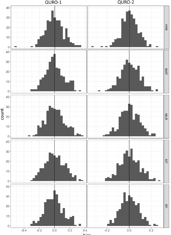
Table 6
Comparison of the performance of five predictive modelling methods for A) QURO_1 and B) QURO_2 sites. Methods were evaluated by 3-fold cross-validation repeated 100 times. The five predictive modelling methods were Multiple Linear Regression (MLR), Artificial Neural Networks (ANN), Model Trees (MT), Bagging of Model Trees (BMT) and Random Forests of Regression Trees (RF). The performance measures were the correlation coefficient (r), root relative squared error (RRSE), root mean squared error (RMSE), index of agreement (d), reduction of error (RE), coefficient of efficiency (CE) and detrended efficiency (DE), calculated on the training (train) and testing (test) data of cross-validation splits. Across the 100 runs of cross-validation, we present the mean, standard deviations (Std), mean rank and share of rank 1 for each performance measure. The best values of each performance measure on the test set are highlighted in bold.
Similarly, as with QURO-1, ANN also had the best validation performance for QURO-2. The second-best performance was obtained by RF, followed by BMT. The worst validation results were recorded for MLR and MT, which performed the best only in 4% (MLR) and 3% (MT) of individual cross-validation splits (Table 6). Histograms of mean bias (Fig. 6) reflect the performance of models from Table 6. The histogram of mean bias for the ANN method shows the best performance, followed by RF and BMT, while the histograms of mean bias for MLR and MT display weaker performance. Based on the results from Table 6 and Fig. 6, the final selected models for both sites would be those learned by ANN.
. Discussion
Climate signal in VLA
The main goal of our study was to compare various regression methods in the task of VLA prediction. To do so, we first analysed the climate signal of VLA chronologies to select predictors for different regression models. The correlation coefficients showed a similar pattern for both sites: the VLA tree-ring parameter was correlated with temperatures at the end of the previous growing season and temperatures at the time of earlywood formation. Many other studies have also reported positive correlations between mean temperatures and VLA (e.g., Fonti and Garcia-Gonzalez, 2008; Garcia-Gonzalez and Fonti, 2008; Matisons and Dauškane, 2009; Tumajer and Treml, 2016).
The April temperature signal is in accordance with xylogenetic studies from similar sites (e.g., Goršić, 2013; Gričar, 2010), which have reported an expansion of earlywood conduits in April. The spring temperature signal stored in vessel characteristics is related to the onset of cambial activity and the duration of the enlargement period before lignification of the vessel secondary wall
(Perez-de-Lis et al., 2016). Rising temperatures before bud break increase the expression of genes involved in polar auxin transport (Schrader et al., 2003), which induces radial growth. The onset of cambial activity starts approximately one month before bud swelling (Gonzalez-Gonzalez et al., 2013; Sass-Klaassen et al., 2011). Earlywood conduits are therefore mainly developed during the period with limited (or no) photosynthetic activity and trees use stored carbohydrates from the previous growing season, leading to the preservation of the temperature signal of the previous growing season in the vessel characteristics.
The correlation coefficients between the sum of monthly precipitation and VLA were negative and significant only for the QURO-1 site, but nevertheless lower than temperature correlations. Negative correlations between VLA and winter precipitation are usually attributed to the excess of water accumulated in the soil (e.g.; González-González et al., 2015). The QURO-1 site is in close proximity to small artificial lakes and water is, therefore, available throughout the year. Water saturation affects anatomical features, mainly the formation of smaller vessels (Ballesteros et al., 2010).
Temperature is, therefore, the most important limiting growth factor at both sites. However, many other studies have reported that earlywood vessel characteristics are mostly related to water availability (Copini et al., 2016; Garcia-Gonzalez and Eckstein, 2003; Garcia-Gonzalez and Fonti, 2008; Kames et al., 2016; St George and Nielsen, 2000). Based on literature published to date, there are no obvious site factors that would explain when VLA is more related to temperature and when to water availability.
Evaluation of various ML algorithms
To the best of our knowledge, our comparative study is the first in the dendroclimatological field to have used VLA tree-ring proxy and several climate predictors to compare different linear and nonlinear methods. In most previous comparative studies with tree-ring and climate data, ANN outperformed MLR (Balybina, 2010; D'Odorico et al., 2000; Jevšenak and Levanič, 2016; Zhang et al., 2000). We confirmed the high predictive abilities of ANN, which outperformed the other regression methods for both sites.
The high performance of nonlinear algorithms might be partially explained by the selection of predictors. By employing months with lower (linear) correlations, such as March and May, we allowed the nonlinear algorithms to use this information and explain the VLA more accurately. April had the strongest linear correlations with VLA at both sites, but temperatures in March and May probably cause nonlinear reactions in VLA. Advanced ML algorithms can use this information and model the relationship between climate and VLA more accurately. ML methods such as ANN should, therefore, become a more standard approach in dendroclimatology.
Despite the obvious outperformance of ANN over all the other regression methods used in our study, we recommend testing several different regression algorithms and selecting the optimal one for climate reconstruction. In a related study, Jevšenak et al. (2017) showed that different datasets favour different regression algorithms and that there is no single method that always outperforms the other regression methods. The methodological approach used in our study to compare different regression methods is implemented in the compare_methods() function from the dendroTools R package (Jevšenak and Levanič, 2018). This function could be used to find the optimal regression method for any dataset, prior to climate reconstruction.
The aggregate expression of the many interacting nonlinear, rate-limited processes within a tree is often effectively a linear response to local climate in its ring widths (Cook and Pederson, 2011). Linearity is, therefore, possible on a smaller part of the entire interval of climate-growth response but, when approaching the edge of this spectrum, the relationship between tree growth and climate is likely to become more or less nonlinear. In addition, in most climate reconstruction models, the reconstruction process estimates data points out of calibration data, i.e., in the spectrum of the climate-tree response, which is expected to react nonlinearly. This is an additional argument in favour of nonlinear methods being used in dendroclimatology, since their predictions are likely to be more accurate.
Our comparative study showed that nonlinear algorithms can provide better models. Machine learning algorithms have several advantages, especially when a number of predictors, with a broader spectrum of climate and tree response data, are considered. In pursuit of more accurate climate reconstructions, it seems reasonable to switch from linear to advanced nonlinear algorithms.
. Conclusions
We analysed the relationship between climate and the VLA parameter and used the results to select predictors to train and compare linear and nonlinear models. The two sites showed very similar results. ANN showed superior results for all mean validation statistics. The second-best models were RF and BMT, followed by MLR and MT. The question of whether it is reasonable to substitute the current gold standard arises. The current gold standard in the field of dendrochronological studies is MLR, but there are alternatives that might provide better predictions. The high performance of ANN was confirmed in our comparative study, but there is no reason to believe that ANN will always outperform other regression methods. We, therefore, suggest implementing our comparison strategy as a standard preliminary process, before using a selected method. To do so, there is a compare_methods() function available in the dendroTools R package.